
I had a bootstrap that needed a lot of replicates, so I moved it onto eight cores. It ran several times faster and returned a different answer every time I called it, which was annoying but at least loud. Then I applied the fix that turns up first in almost every search, the code became perfectly reproducible, and it kept quietly throwing away seven eighths of the work it was doing.
The rule that stops holding is simple once you see it. set.seed() seeds one random number stream inside one R process, and parallel workers are separate processes. The seed you set on the master never reaches them, so whatever the workers do about randomness, they do on their own.
Below I take a real question that genuinely needs many replicates, break it three different ways, measure what each break costs, and end with the seeding that still gives the same answer on a machine with a different number of cores.
A question with an uncertain answer
I am using nycflights13, which ships every flight that left the three New York airports in 2013. The question is about the tail rather than the average: for each carrier, how late is a bad arrival? I take the 90th percentile of arrival delay, and I keep the carriers with at least 500 flights so that a percentile means something.
library(dplyr)
library(tidyr)
library(ggplot2)
library(nycflights13)

delays <- flights |>
  filter(!is.na(arr_delay)) |>
  select(carrier, arr_delay)

keep <- delays |> count(carrier) |> filter(n >= 500) |> pull(carrier)
delays <- delays |> filter(carrier %in% keep)

by_carrier <- split(delays$arr_delay, delays$carrier)

observed <- by_carrier |>
  vapply(function(x) quantile(x, 0.9, names = FALSE), numeric(1))

tibble(carrier = names(observed), q90 = observed, n = lengths(by_carrier)) |>
  arrange(desc(q90)) |>
  head(5)
## # A tibble: 5 × 3
##   carrier   q90     n
##   <chr>   <dbl> <int>
## 1 EV       77   51108
## 2 F9       76     681
## 3 YV       76     544
## 4 FL       69.6  3175
## 5 9E       64   17294
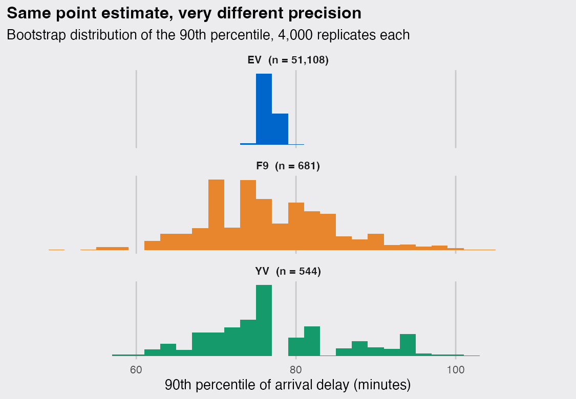
Three carriers sit on top within one minute of each other, and their sample sizes are not remotely comparable. EV has 51,108 flights behind its estimate, while F9 has 681 and YV has 544. A ranking read straight off those point estimates would be reporting sampling noise as a result.
A bootstrap fixes that. Since the comparison is between carriers, I resample within each carrier and keep its number of flights fixed, which is the stratified version and the one that carries each carrier’s own sample size into the answer.
boot_q90 <- function(i) {
  vapply(by_carrier,
         function(x) quantile(sample(x, length(x), replace = TRUE), 0.9, names = FALSE),
         numeric(1))
}

R <- 4000
serial_time <- system.time({
  set.seed(42)
  reps <- do.call(rbind, lapply(seq_len(R), boot_q90))
})
dim(reps)
## [1] 4000   14
dsp_colors <- c("#0066CC", "#E8862D", "#159A6C", "#7D5BD6",
                "#D64580", "#2AA9B8", "#C9A227")
dsp_theme <- theme_minimal(base_size = 13) +
  theme(plot.background    = element_rect(fill = "#ECECEF", color = NA),
        panel.background   = element_rect(fill = "#ECECEF", color = NA),
        panel.grid.minor   = element_blank(),
        panel.grid.major.y = element_blank(),
        panel.grid.major.x = element_line(color = "grey78"),
        axis.ticks         = element_blank(),
        plot.title         = element_text(face = "bold"),
        strip.text         = element_text(face = "bold"))

intervals <- as_tibble(t(apply(reps, 2, quantile, c(0.025, 0.975))), rownames = "carrier") |>
  rename(lo = `2.5%`, hi = `97.5%`) |>
  mutate(q90 = observed[carrier], n = lengths(by_carrier)[carrier])

ggplot(intervals, aes(q90, reorder(carrier, q90))) +
  geom_linerange(aes(xmin = lo, xmax = hi), color = dsp_colors[1], linewidth = 1) +
  geom_point(size = 2.4, color = dsp_colors[1]) +
  geom_text(aes(x = hi, label = paste0("n = ", format(n, big.mark = ",", trim = TRUE))),
            hjust = -0.15, size = 3.2, color = "grey35") +
  scale_x_continuous(limits = c(15, 108)) +
  labs(title = "Tail delay by carrier, with bootstrap uncertainty",
       subtitle = "90th percentile of arrival delay, 95% bootstrap interval",
       x = "90th percentile of arrival delay (minutes)", y = NULL) +
  dsp_theme
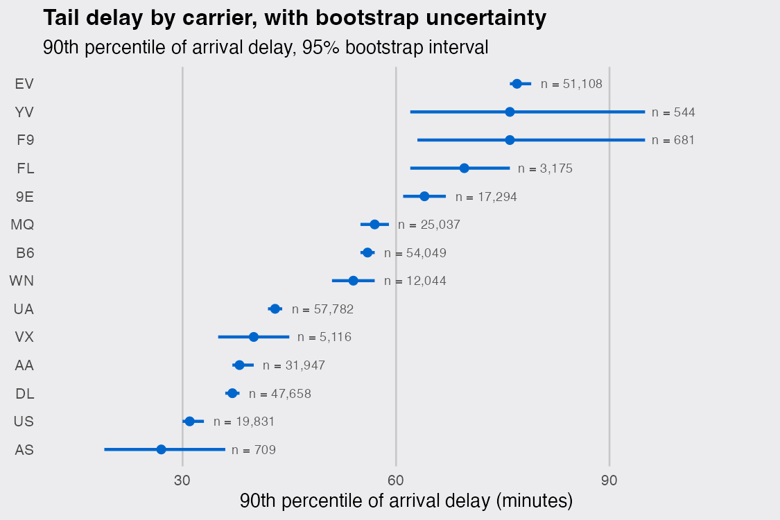
The top of that chart is a three way tie held up by two very different amounts of evidence. EV’s interval is three minutes wide and F9’s is more than thirty, so they are the same estimate in name only.
top3 <- c("EV", "F9", "YV")
labels <- setNames(paste0(top3, "  (n = ",
                          format(lengths(by_carrier)[top3], big.mark = ",", trim = TRUE), ")"),
                   top3)

as_tibble(reps[, top3]) |>
  pivot_longer(everything(), names_to = "carrier", values_to = "q90") |>
  mutate(carrier = factor(labels[carrier], levels = labels)) |>
  ggplot(aes(q90, fill = carrier)) +
  geom_histogram(binwidth = 2, show.legend = FALSE) +
  facet_wrap(~carrier, ncol = 1, scales = "free_y") +
  scale_fill_manual(values = dsp_colors[1:3]) +
  labs(title = "Same point estimate, very different precision",
       subtitle = paste("Bootstrap distribution of the 90th percentile,",
                        format(R, big.mark = ","), "replicates each"),
       x = "90th percentile of arrival delay (minutes)", y = NULL) +
  dsp_theme + theme(axis.text.y = element_blank())
So instead of ranking the point estimates, I ask the bootstrap directly how often each carrier comes out worst.
p_worst <- function(m) {
  winners <- factor(colnames(m)[max.col(m, ties.method = "first")], levels = colnames(m))
  prop.table(table(winners))
}

round(sort(p_worst(reps), decreasing = TRUE)[1:4], 3)
## winners
##    EV    F9    YV    FL
## 0.362 0.336 0.299 0.004
That is the honest answer: the worst carrier for tail delay in 2013 is undecided between three of them, with EV at 36%, F9 at 34% and YV at 30%. It is also the kind of answer that needs a lot of replicates, because it is a probability, and the Monte Carlo error on a probability near 0.36 only falls with the square root of the replicate count.
Going parallel
The serial run took 67 seconds for 4,000 replicates. That is tolerable here, and it stops being tolerable as soon as the statistic is a model fit rather than a quantile, or the replicate count goes up an order of magnitude. Resampling is embarrassingly parallel, so the obvious move is a cluster.
library(parallel)

W <- 8
cl <- makeCluster(W)
clusterExport(cl, "by_carrier")
## Error in `get()`:
## ! object 'by_carrier' not found
par_time <- system.time({
  set.seed(1)
  run_a <- do.call(rbind, parLapply(cl, seq_len(R), boot_q90))
})

set.seed(1)
run_b <- do.call(rbind, parLapply(cl, seq_len(R), boot_q90))

identical(run_a, run_b)
## [1] FALSE
clusterExport() is needed because the workers are fresh R processes that have never seen my data. The seed is the same story, and it does not have an export step. set.seed(1) seeded the master, the workers were never told, and two runs of identical code disagree.
The wall clock did improve: 11.1 seconds against 67, a speedup of about 6.1 times on 8 workers. The result is just not the same twice, which for a bootstrap that other people are meant to be able to check is not a result at all.
mclapply() behaves the same way from the user’s point of view, for a different internal reason. Its mc.set.seed = TRUE default gives each forked child a seed derived from its process id and the clock, so the children differ from each other, and the whole job differs from run to run. It also only forks on macOS and Linux.
The fix that makes it reproducible
The natural repair is to seed the workers, since the workers are the ones drawing the numbers. One clusterEvalQ() call does it, and it works.
invisible(clusterEvalQ(cl, set.seed(123)))
shared_a <- do.call(rbind, parLapply(cl, seq_len(R), boot_q90))

invisible(clusterEvalQ(cl, set.seed(123)))
shared_b <- do.call(rbind, parLapply(cl, seq_len(R), boot_q90))

identical(shared_a, shared_b)
## [1] TRUE
Reproducible. Same code, same seed, same numbers, and every check I would normally run on a parallel script now passes. Here is the check I did not think to run.
nrow(unique(shared_a))
## [1] 501
501 distinct replicates out of 4,000. parLapply() splits 1:4000 into 8 contiguous chunks and hands one to each worker, every worker starts from the state set.seed(123) put it in, and boot_q90() ignores its index argument because a bootstrap replicate does not depend on which replicate it is. So every worker walked the same random stream and drew the same resamples, and the 4,000 rows hold nothing but repeats of the 501 the longest chunk got through.
Nothing warned. The job took the same time as before, filled a matrix of the right shape, and produced a number that looks exactly like the number I asked for.
What the duplicates cost
Duplicating every replicate the same number of times does not bias anything, since the mean and the quantiles of the stack are the mean and quantiles of the unique part. What it destroys is precision. I paid for 4,000 replicates and I am holding the Monte Carlo error of 501.
To see it rather than argue it, I run the whole bootstrap twelve times under each scheme, changing only the seed, and watch how much the answer moves. The correct scheme here is clusterSetRNGStream(), which I come back to in a moment.
library(purrr)

run_scheme <- function(scheme, seed) {
  if (scheme == "shared") {
    invisible(clusterCall(cl, function(s) set.seed(s), seed))
  } else {
    clusterSetRNGStream(cl, seed)
  }
  do.call(rbind, parLapply(cl, seq_len(R), boot_q90))
}

stability <- expand_grid(seed = 1:12, scheme = c("shared", "stream")) |>
  pmap(function(seed, scheme) {
    shares <- p_worst(run_scheme(scheme, seed))
    tibble(seed = seed, scheme = scheme,
           carrier = names(shares), p = as.numeric(shares))
  }) |>
  list_rbind()
spread <- stability |>
  filter(carrier %in% c("EV", "F9", "YV")) |>
  group_by(scheme, carrier) |>
  summarise(sd = sd(p), lowest = min(p), highest = max(p), .groups = "drop")

spread |> mutate(across(sd:highest, \(x) round(x, 3)))
## # A tibble: 6 × 5
##   scheme carrier    sd lowest highest
##   <chr>  <chr>   <dbl>  <dbl>   <dbl>
## 1 shared EV      0.022  0.342   0.428
## 2 shared F9      0.019  0.29    0.345
## 3 shared YV      0.017  0.277   0.338
## 4 stream EV      0.007  0.36    0.381
## 5 stream F9      0.009  0.314   0.342
## 6 stream YV      0.008  0.294   0.32
stability |>
  filter(carrier %in% c("EV", "F9", "YV")) |>
  mutate(scheme = factor(ifelse(scheme == "shared",
                                "one seed, set inside each worker",
                                "clusterSetRNGStream()"),
                         levels = c("one seed, set inside each worker",
                                    "clusterSetRNGStream()"))) |>
  ggplot(aes(p, scheme, color = scheme)) +
  geom_point(size = 2.6, alpha = 0.8, show.legend = FALSE) +
  facet_wrap(~carrier, ncol = 1) +
  scale_color_manual(values = dsp_colors[c(2, 1)]) +
  scale_x_continuous(labels = \(x) paste0(round(100 * x), "%")) +
  labs(title = "Same wall clock, a fraction of the precision",
       subtitle = paste("Bootstrap probability of ranking worst, 12 runs at",
                        format(R, big.mark = ","), "replicates"),
       x = "estimated probability of ranking worst", y = NULL) +
  dsp_theme
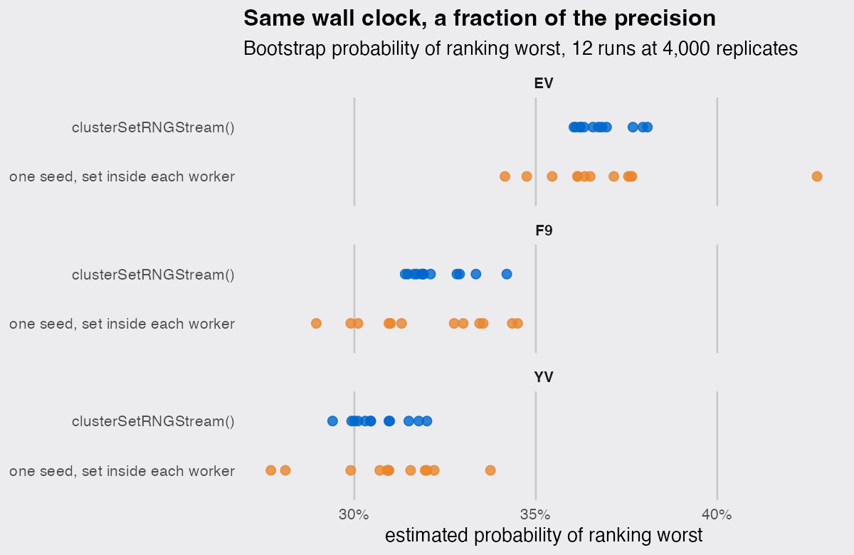
Across twelve seeds, the probability that EV ranks worst lands between 36% and 38% with proper streams, and between 34% and 43% with the shared seed. The standard deviations are 0.0072 and 0.0217, a ratio of 3.
That ratio is not a coincidence, and it is the cleanest confirmation that the duplicates are exactly as expensive as they look. For a proportion near 0.36, the Monte Carlo standard error is 0.0076 at 4,000 replicates and 0.0215 at 501. The two observed spreads are 0.0072 and 0.0217. The shared seed run behaves like what it is, a 501 replicate bootstrap wearing a 4,000 replicate label, at 8 times the compute.
Seeding parallel R properly
The thing worth taking away is that the fix is never "call set.seed() somewhere else". It is to give each worker a stream that is guaranteed not to overlap with any other worker’s, which is what L’Ecuyer’s combined multiple recursive generator is for. Base R has had this built in for years.
clusterSetRNGStream(cl, 123)
stream_a <- do.call(rbind, parLapply(cl, seq_len(R), boot_q90))

clusterSetRNGStream(cl, 123)
stream_b <- do.call(rbind, parLapply(cl, seq_len(R), boot_q90))

identical(stream_a, stream_b)
## [1] TRUE
nrow(unique(stream_a))
## [1] 4000
Reproducible and 4,000 distinct replicates, which is the combination the shared seed could not give me. One call, before the work, and the master’s own seed is left untouched.
If you work in the futureverse, furrr asks you for the seed rather than letting you forget it. Calling future_map() on code that draws random numbers without a seed raises an UNRELIABLE VALUE warning, which is the loudest any of these tools gets about the problem.
library(furrr)

plan(multisession, workers = W)
furrr_a <- do.call(rbind, future_map(seq_len(R), boot_q90,
                                     .options = furrr_options(seed = 123)))
furrr_b <- do.call(rbind, future_map(seq_len(R), boot_q90,
                                     .options = furrr_options(seed = 123)))

identical(furrr_a, furrr_b)
## [1] TRUE
nrow(unique(furrr_a))
## [1] 4000
For foreach, the operator to reach for is %dorng% from doRNG, or a registerDoRNG() call that upgrades every %dopar% in the session. Plain %dopar% with doParallel has the same problem as plain parLapply().
library(foreach)
library(doParallel)
library(doRNG)

registerDoParallel(cl)
registerDoRNG(123)
rng_a <- foreach(i = seq_len(R), .combine = rbind) %dopar% boot_q90(i)
registerDoRNG(123)
rng_b <- foreach(i = seq_len(R), .combine = rbind) %dopar% boot_q90(i)

identical(unname(rng_a), unname(rng_b))
## [1] TRUE
nrow(unique(rng_a))
## [1] 4000
Per worker streams or per replicate seeds
All three of those are correct, and they are not the same kind of correct. That difference caught me out, and it is the part I would most want to know in advance.
clusterSetRNGStream() hands one stream to each worker. The replicates a worker produces therefore depend on how many workers there are, because the chunk it receives and the stream it holds both change. furrr and doRNG work the other way and generate one seed per element of the loop up front, so a replicate carries its own seed regardless of who runs it.
small <- 200

with_workers <- function(w, f) {
  cl2 <- makeCluster(w); on.exit(stopCluster(cl2))
  clusterExport(cl2, "by_carrier")
  f(cl2)
}

stream_8 <- with_workers(8, \(cl2) { clusterSetRNGStream(cl2, 123)
  do.call(rbind, parLapply(cl2, seq_len(small), boot_q90)) })
## Error in `get()`:
## ! object 'by_carrier' not found
stream_2 <- with_workers(2, \(cl2) { clusterSetRNGStream(cl2, 123)
  do.call(rbind, parLapply(cl2, seq_len(small), boot_q90)) })
## Error in `get()`:
## ! object 'by_carrier' not found
plan(multisession, workers = 8)
furrr_8 <- do.call(rbind, future_map(seq_len(small), boot_q90, .options = furrr_options(seed = 123)))
plan(multisession, workers = 2)
furrr_2 <- do.call(rbind, future_map(seq_len(small), boot_q90, .options = furrr_options(seed = 123)))
plan(sequential)
furrr_1 <- do.call(rbind, future_map(seq_len(small), boot_q90, .options = furrr_options(seed = 123)))

c(stream_8_vs_2 = identical(stream_8, stream_2),
  furrr_8_vs_2  = identical(furrr_8, furrr_2),
  furrr_8_vs_seq = identical(furrr_8, furrr_1))
## Error:
## ! object 'stream_8' not found
So a script seeded with clusterSetRNGStream() is reproducible on my machine and stops being reproducible on a laptop with four cores instead of eight, or on a server where someone bumped the worker count to speed things up. A script seeded per replicate returns the same numbers on eight workers, on two, and with no parallelism at all. If the result is going into a paper or a report that someone else has to rerun, that invariance is worth more than the small overhead of generating the seeds up front.
The check to run on your own code
The diagnostic that would have caught all of this fits on one line, so it is worth running once on any resampling job you have already parallelized.
nrow(unique(replicates)) # or dplyr::n_distinct() on a vector of statistics
If that comes back equal to your replicate count, the streams are fine. If it comes back near replicates divided by workers, every worker is drawing the same numbers and you are paying full price for a fraction of the answer. The count is worth keeping in the script rather than running once, because it costs nothing and it fails loudly on the day someone changes how the job is launched.
The wider version of the lesson is that reproducibility and randomness are separate properties, and parallel code can satisfy one while destroying the other. A run that gives the same answer twice has told you nothing about whether the numbers inside it were drawn independently. That is the check the seed was supposed to imply, and going parallel is exactly where it stops being implied.
