
When the price of gasoline goes up, the pump seems to follow overnight; when it comes down, the pump seems to take its time. Economists call this "rockets and feathers", and I wanted to measure it with nothing but public weekly prices and a regression. Since 2020, US pump prices have passed on 60% of a rise in the wholesale price of gasoline by the following Monday, and 18% of a fall. A week later it is 82% against 41%, and the gap takes about three weeks to close. Before 2020 the gap was smaller and gone within a week. One step earlier there is no gap at all: 90% of a rise in crude oil and 91% of a fall reach the wholesale gasoline price in the same week. The slow part is the last step, from the wholesale market to the pump.
How do I estimate asymmetric price pass-through in R?
Split the weekly change in the input price into its rises and its falls with pmax() and pmin(), regress the weekly change in the output price on the current and lagged values of both, and add the coefficients up week by week. Each running sum is the share of a one-cent change that has reached the output price after that many weeks, and comparing the sum for rises with the sum for falls is the test. The block below runs on its own with httr2 1.3.0, sandwich 3.1.3 and dplyr 1.2.1 on R 4.6.1. It uses two weekly series from FRED: the US average pump price of regular gasoline (GASREGW, taxes included) and the wholesale spot price of regular gasoline in New York Harbor (WGASNYH), both in dollars per gallon.
library(tidyverse)
library(httr2)      # as of October 2026, FRED refuses R's default user agent
library(sandwich)   # Newey-West standard errors

fred <- function(id, shift = 0) {
  request("https://fred.stlouisfed.org/graph/fredgraph.csv") |>
    req_url_query(id = id) |>
    req_perform() |>
    resp_body_string() |>
    I() |>
    read_csv(show_col_types = FALSE) |>
    set_names(c("date", "value")) |>
    mutate(date = date + shift)
}

# Pump prices are surveyed at 8am Monday; wholesale prices are the average of
# the week ending the Friday before, so move them forward three days to line up
prices <- inner_join(fred("GASREGW"), fred("WGASNYH", shift = 3),
                     by = "date", suffix = c("_pump", "_wholesale"))

pass_through <- function(data, out, inp, weeks = 10, years = c(1990, 2026)) {
  d <- data |>
    arrange(date) |>
    mutate(d_out = {{ out }} - lag({{ out }}),   # weekly change, dollars/gallon
           d_in  = {{ inp }} - lag({{ inp }}))
  for (k in 0:weeks) {                           # rises and falls, lagged 0..weeks
    d[[paste0("rise_", k)]] <- lag(pmax(d$d_in, 0), k)
    d[[paste0("fall_", k)]] <- lag(pmin(d$d_in, 0), k)
  }
  d <- filter(d, between(year(date), years[1], years[2]))
  fit <- lm(d_out ~ ., data = select(d, d_out, starts_with(c("rise_", "fall_"))))
  b <- coef(fit)
  V <- NeweyWest(fit)                            # weekly errors are autocorrelated
  map(0:weeks, \(j) {
    rise <- names(b) %in% paste0("rise_", 0:j)   # sum the coefficients for weeks 0..j
    fall <- names(b) %in% paste0("fall_", 0:j)
    W <- rbind(rise, fall, gap = rise - fall)
    tibble(week = j, move = rownames(W),
           share = drop(W %*% b), se = sqrt(diag(W %*% V %*% t(W))))
  }) |> list_rbind()
}

all_years <- pass_through(prices, value_pump, value_wholesale)
all_years |>
  filter(week <= 3) |>
  pivot_wider(id_cols = week, names_from = move, values_from = share)
## # A tibble: 4 × 4
##    week  rise  fall     gap
##   <int> <dbl> <dbl>   <dbl>
## 1     0 0.565 0.295 0.271
## 2     1 0.731 0.553 0.178
## 3     2 0.786 0.691 0.0954
## 4     3 0.813 0.807 0.00600
The pump price is a survey of about 900 stations at 8 am on Monday, and the wholesale price is the average of the trading days in the week to the Friday before, so shifting the wholesale date forward three days pairs each Monday with the most recent week the stations had seen. Over all 1,882 weeks from August 1990 to September 2026, 57% of a wholesale rise is at the pump by the next Monday against 29% of a fall, so rises move 1.9 times as fast in the first week. By the third week the two sums are level, at 81% and 81%. The standard errors come from NeweyWest() because weekly price changes are autocorrelated, which makes the plain lm() errors too narrow. Fit the usual symmetric version instead, with a single coefficient per week, and the first-week answer is 44%: an average of two speeds that describes neither.
Where the delay happens, and when it grew
The same function runs on the step before, Brent crude oil (WCOILBRENTEU, converted from dollars per barrel at 42 gallons to the barrel) into wholesale gasoline, and on the retail step split at 2020:
crude <- fred("WCOILBRENTEU", shift = 3) |>
  mutate(value = value / 42)                     # dollars per barrel -> per gallon
refinery <- inner_join(fred("WGASNYH", shift = 3), crude,
                       by = "date", suffix = c("_wholesale", "_crude"))

stages <- bind_rows(
  "Crude to wholesale, 1990-2026" = pass_through(refinery, value_wholesale, value_crude),
  "Wholesale to pump, 1990-2019"  = pass_through(prices, value_pump, value_wholesale, years = c(1990, 2019)),
  "Wholesale to pump, 2020-2026"  = pass_through(prices, value_pump, value_wholesale, years = c(2020, 2026)),
  .id = "stage") |>
  mutate(stage = fct_inorder(stage))
dsp_colors <- c("#0066CC", "#E8862D", "#159A6C", "#7D5BD6",
                "#D64580", "#2AA9B8", "#C9A227")
dsp_theme <- theme_minimal(base_size = 13) +
  theme(plot.background    = element_rect(fill = "#ECECEF", color = NA),
        panel.background   = element_rect(fill = "#ECECEF", color = NA),
        panel.grid.minor   = element_blank(),
        panel.grid.major.x = element_blank(),
        panel.grid.major.y = element_line(color = "grey78"),
        axis.ticks         = element_blank(),
        plot.title         = element_text(face = "bold"),
        strip.text         = element_text(face = "bold"))

stages |>
  filter(move != "gap") |>
  mutate(move = if_else(move == "rise", "Price rises", "Price falls")) |>
  ggplot(aes(week, share, color = move, fill = move)) +
  geom_hline(yintercept = 1, color = "grey45") +
  geom_ribbon(aes(ymin = share - 1.96 * se, ymax = share + 1.96 * se),
              alpha = 0.18, color = NA) +             # 95% intervals
  geom_line(linewidth = 1) +
  geom_point(size = 1.6) +
  facet_wrap(~ stage) +
  scale_x_continuous(breaks = seq(0, 10, 2)) +
  scale_y_continuous(labels = scales::label_percent(), breaks = seq(0, 1.25, 0.25)) +
  scale_color_manual(values = c("Price rises" = dsp_colors[2], "Price falls" = dsp_colors[1]),
                     breaks = c("Price rises", "Price falls")) +
  scale_fill_manual(values = c("Price rises" = dsp_colors[2], "Price falls" = dsp_colors[1]),
                    breaks = c("Price rises", "Price falls")) +
  labs(x = "Weeks after the price change", y = "Share passed on so far",
       color = NULL, fill = NULL) +
  dsp_theme +
  theme(legend.position = "top")
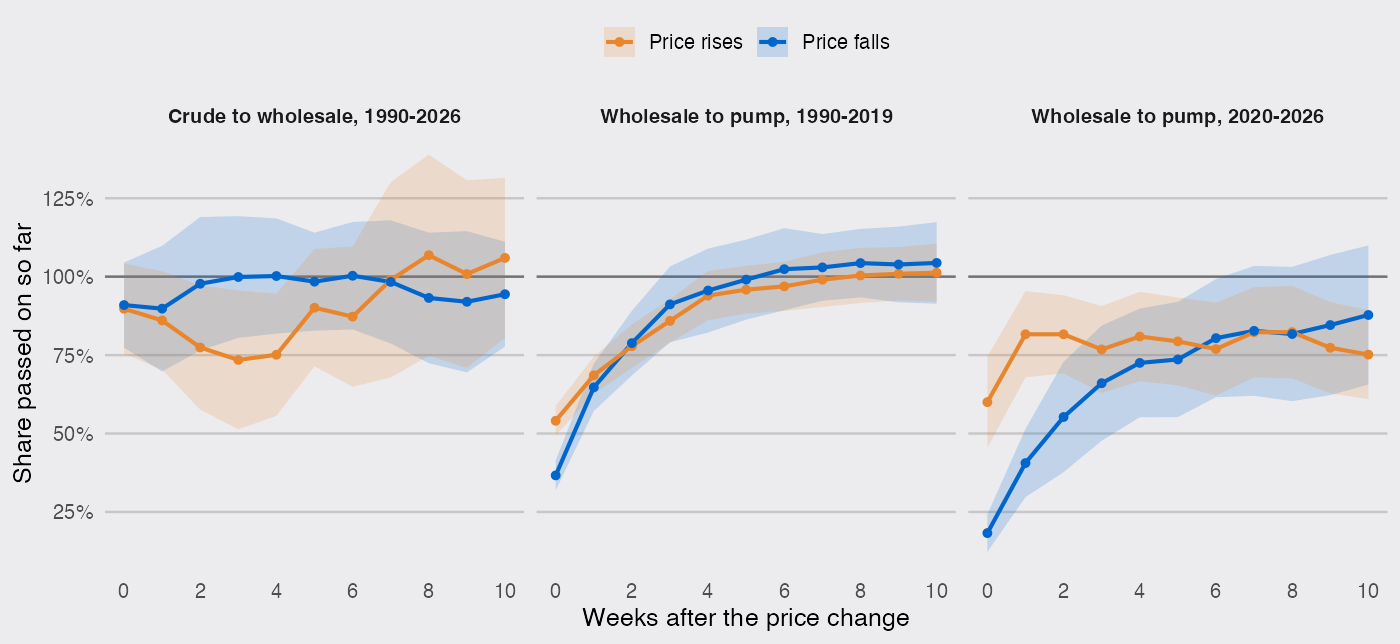
In the crude oil step, 90% of a rise and 91% of a fall reach wholesale gasoline within the week, and the two intervals overlap at every lag. Whatever slows the falls down, it is not the wholesale market.
The retail step is a different picture, and it changed around 2020. Before then, a wholesale rise put 54% on the pump by Monday and a fall 37%, and a week later the sums were 69% and 65%. Since 2020 the first week is 60% against 18%, a gap with a 95% interval of 23 to 60 percentage points, and by the third week it has narrowed to 11 points, no longer distinguishable from zero. In cents: since 2020, a 10-cent wholesale rise has added 6.0 cents at the pump by the next Monday and 8.2 by the Monday after, while a 10-cent fall has taken off 1.8 and 4.1. Using Gulf Coast wholesale prices (WGASUSGULF) instead of New York Harbor gives the same 2020-2026 split, 59% against 18% in the first week. From the sixth week on the two curves cross and sit inside each other’s intervals, so the asymmetry is about how fast a change arrives, not how much of it eventually does.
The calendar-week join that hides it
The three-day shift matters more than it looks. Join the two series by calendar week instead, the way floor_date() or tsibble’s yearweek() would group them, and each Monday pump price is paired with the wholesale average of the days that come after it:
same_week <- inner_join(
  fred("GASREGW") |> mutate(cal_week = floor_date(date, "week")),
  fred("WGASNYH") |> mutate(cal_week = floor_date(date, "week")) |> select(-date),
  by = "cal_week", suffix = c("_pump", "_wholesale"))

wrong <- pass_through(same_week, value_pump, value_wholesale)
Now 6% of a rise and 2% of a fall reach the pump in the first week, and the gap between rises and falls appears to open a week later (62% against 31%). Read at face value, stations ignore wholesale prices for a week. Nothing in the output flags the problem: the regression is relating each Monday’s pump price to wholesale prices that did not exist yet when it was recorded.
Falls do reach the pump; since 2020 they have just spent about three weeks behind rises before the difference fades. Weekly national averages cannot say why; the explanations on offer range from drivers shopping around harder while prices climb to stations rebuilding margins while costs fall, and telling them apart takes station-level prices. What the public series do show is where the delay sits: not between crude oil and wholesale gasoline, which move together in both directions, but in the last step to the pump.

