Results so far obtained allow us to predict the RainTomorrow Yes/No variable. In the first part, we highlighted that such factor variable can be put in relationship with the Rainfall quantitative one by:
all.equal(weather_data$Rainfall > 1, weather_data$RainToday == "Yes")
As a consequence, we are able so far to predict if tomorrow rainfall shall be above 1mm or not. Some more questions to be answered:
- In case of “at least moderate” Rainfall (arbitrarily defined as Rainfall > 15mm), how do our models perform?
In case of “at least moderate” rainfall, we would like to be as much reliable as possible in predicting {RainTomorrow = “Yes”}. Since RainTomorrow = “Yes” is perceived as the prediction of a potential threat of damages due to the rainfall, we have to alert Canberra’s citizens properly. That translates in having a very good specificity, as explained in the presecution of the analysis.
- Can we build additional models in order to predict further variables such as tomorrow’s Rainfall, Humidity3pm, WindGustSpeed, Sunshine, MinTemp and MaxTemp variables?
That is motivated by the fact that weather forecast comprises more than one prediction. For an example of the most typical ones, see:
Moderate Rainfall Scenario
Since Rainfall was one of the variable we drop off from our original dataset, we have to consider it back and identify the records which are associated to moderate rainfall. The following note applies.
Note on predictors availability
In the prosecution of the analysis, we will not make the assumption to have to implement separate 9AM, 3PM and late evening predictions as done in part #2. For simplicity and brevity, we assume to have to arrange this new goals in the late evening where all predictors are available. Similarly as done before, we will not take into account the following variables:
Date, Location, RISK_MM, RainToday, Rainfall, WindDir9am, WindDir3pm
as Date and Location cannot be used as predictors; RISK_MM, RainToday, Rainfall are not used to make our task a little bit more difficult; we demonstrated in the first tutorial of this series that WinDir9am and WinDir3pm are not interesting predictors and they have associated a considerable number of NA values.
Having said that, we then start the moderate rainfall scenario analysis. At the same time, we prepare the dataset for the rest of the analysis.
weather_data6 <- subset(weather_data, select = -c(Date, Location, RISK_MM, RainToday, WindDir9am, WindDir3pm))
weather_data6$RainfallTomorrow <- c(weather_data6$Rainfall[2:nrow(weather_data6)], NA)
weather_data6$Humidity3pmTomorrow <- c(weather_data6$Humidity3pm[2:nrow(weather_data6)], NA)
weather_data6$WindGustSpeedTomorrow <- c(weather_data6$WindGustSpeed[2:nrow(weather_data6)], NA)
weather_data6$SunshineTomorrow <- c(weather_data6$Sunshine[2:nrow(weather_data6)], NA)
weather_data6$MinTempTomorrow <- c(weather_data6$MinTemp[2:nrow(weather_data6)], NA)
weather_data6$MaxTempTomorrow <- c(weather_data6$MaxTemp[2:nrow(weather_data6)], NA)

weather_data7 = weather_data6[complete.cases(weather_data6),]
head(weather_data7)
 MinTemp MaxTemp Rainfall Evaporation Sunshine WindGustDir WindGustSpeed WindSpeed9am WindSpeed3pm
1     8.0    24.3      0.0         3.4      6.3          NW            30            6           20
2    14.0    26.9      3.6         4.4      9.7         ENE            39            4           17
3    13.7    23.4      3.6         5.8      3.3          NW            85            6            6
4    13.3    15.5     39.8         7.2      9.1          NW            54           30           24
5     7.6    16.1      2.8         5.6     10.6         SSE            50           20           28
6     6.2    16.9      0.0         5.8      8.2          SE            44           20           24
  Humidity9am Humidity3pm Pressure9am Pressure3pm Cloud9am Cloud3pm Temp9am Temp3pm RainTomorrow
1          68          29      1019.7      1015.0        7        7    14.4    23.6          Yes
2          80          36      1012.4      1008.4        5        3    17.5    25.7          Yes
3          82          69      1009.5      1007.2        8        7    15.4    20.2          Yes
4          62          56      1005.5      1007.0        2        7    13.5    14.1          Yes
5          68          49      1018.3      1018.5        7        7    11.1    15.4           No
6          70          57      1023.8      1021.7        7        5    10.9    14.8           No
  RainfallTomorrow Humidity3pmTomorrow WindGustSpeedTomorrow SunshineTomorrow MinTempTomorrow
1              3.6                  36                    39              9.7            14.0
2              3.6                  69                    85              3.3            13.7
3             39.8                  56                    54              9.1            13.3
4              2.8                  49                    50             10.6             7.6
5              0.0                  57                    44              8.2             6.2
6              0.2                  47                    43              8.4             6.1
  MaxTempTomorrow
1            26.9
2            23.4
3            15.5
4            16.1
5            16.9
6            18.2
hr_idx = which(weather_data7$RainfallTomorrow > 15)
It is important to understand what is the segmentation of moderate rainfall records in terms of training and testing set, as herein shown.
(train_hr <- hr_idx[hr_idx %in% train_rec])
[1]   9  22  30  52  79 143 311
(test_hr <- hr_idx[!(hr_idx %in% train_rec)])
[1]   3  99 239 251
We see that some of the “at least moderate” Rainfall records belong to the testing dataset, hence we can use it in order to have a measure based on unseen data by our model. We test the evening models with a test-set comprising such moderate rainfall records.
rain_test <- weather_data7[test_hr,]
rain_test
  MinTemp MaxTemp Rainfall Evaporation Sunshine WindGustDir WindGustSpeed WindSpeed9am WindSpeed3pm
3      13.7    23.4      3.6         5.8      3.3          NW            85            6            6
99     14.5    24.2      0.0         6.8      5.9         SSW            61           11           20
250     3.0    11.1      0.8         1.4      0.2           W            35            0           13
263    -1.1    11.0      0.2         1.8      0.0         WNW            41            0            6
    Humidity9am Humidity3pm Pressure9am Pressure3pm Cloud9am Cloud3pm Temp9am Temp3pm RainTomorrow
3            82          69      1009.5      1007.2        8        7    15.4    20.2          Yes
99           76          76       999.4       998.9        7        7    17.9    20.3          Yes
250          99          96      1024.4      1021.1        7        8     6.3     8.6          Yes
263          92          87      1014.4      1009.0        7        8     2.4     8.7          Yes
    RainfallTomorrow Humidity3pmTomorrow WindGustSpeedTomorrow SunshineTomorrow MinTempTomorrow
3               39.8                  56                    54              9.1            13.3
99              16.2                  58                    41              5.6            12.4
250             16.8                  72                    35              6.5             2.9
263             19.2                  56                    54              7.5             2.3
    MaxTempTomorrow
3              15.5
99             19.9
250             9.5
263            11.6
Let us see how the first weather forecast evening model performs.
opt_cutoff <- 0.42
pred_test <- predict(mod_ev_c2_fit, rain_test, type="prob")
prediction <- as.factor(ifelse(pred_test$Yes >= opt_cutoff, "Yes", "No"))
data.frame(prediction = prediction, RainfallTomorrow = rain_test$RainfallTomorrow)
 prediction RainfallTomorrow
1        Yes             39.8
2         No             16.2
3        Yes             16.8
4        Yes             19.2
confusionMatrix(prediction, rain_test$RainTomorrow)
Confusion Matrix and Statistics

          Reference
Prediction No Yes
       No   0   1
       Yes  0   3

               Accuracy : 0.75
                 95% CI : (0.1941, 0.9937)
    No Information Rate : 1
    P-Value [Acc > NIR] : 1

                  Kappa : 0
 Mcnemar's Test P-Value : 1

            Sensitivity :   NA
            Specificity : 0.75
         Pos Pred Value :   NA
         Neg Pred Value :   NA
             Prevalence : 0.00
         Detection Rate : 0.00
   Detection Prevalence : 0.25
      Balanced Accuracy :   NA

       'Positive' Class : No
Then, the second evening weather forecast model.
opt_cutoff <- 0.56
pred_test <- predict(mod_ev_c3_fit, rain_test, type="prob")
prediction <- as.factor(ifelse(pred_test$Yes >= opt_cutoff, "Yes", "No"))
data.frame(prediction = prediction, RainfallTomorrow = rain_test$RainfallTomorrow)
  prediction RainfallTomorrow
1        Yes             39.8
2        Yes             16.2
3         No             16.8
4        Yes             19.2
confusionMatrix(prediction, rain_test$RainTomorrow)
Confusion Matrix and Statistics

          Reference
Prediction No Yes
       No   0   1
       Yes  0   3

               Accuracy : 0.75
                 95% CI : (0.1941, 0.9937)
    No Information Rate : 1
    P-Value [Acc > NIR] : 1

                  Kappa : 0
 Mcnemar's Test P-Value : 1

            Sensitivity :   NA
            Specificity : 0.75
         Pos Pred Value :   NA
         Neg Pred Value :   NA
             Prevalence : 0.00
         Detection Rate : 0.00
   Detection Prevalence : 0.25
      Balanced Accuracy :   NA

       'Positive' Class : No
For both evening forecast models, one of the testing set predictions is wrong. If we like to improve it, we have to step back to the tuning procedure and determine a decision threshold value more suitable to capture such scenarios. From the tables that we show in the previous part, we can try to lower the cutoff value to increase specificity, however likely implying to reduce accuracy.
Chance of Rain
In the previous part of this series, when discussing with the tuning of the decision threshold, we dealt with probabilities associated to the predicted RainTomorrow variable. The chances of having RainTomorrow == “Yes” are equivalent to the chance of rain. Hence the following utility function can be depicted at the purpose
chance_of_rain <- function(model, data_record){
   chance_frac <- predict(mod_ev_c3_fit, data_record, type="prob")[, "Yes"]
   paste(round(chance_frac*100), "%", sep="")
}
We try it out passing ten records of the testing dataset.
chance_of_rain(mod_ev_c3_fit, testing[1:10,])
[1] "79%" "3%"  "4%"  "3%"  "1%"  "7%"  "69%" "61%" "75%" "78%"
To build all the following models, we are going to use all the data available in order to capture the variability of an entire year. For brevity, we do not make comparison among models for same predicted variable and we do not show regression models diagnostic plots.
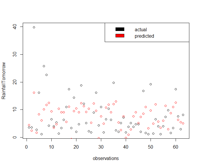
Tomorrow’s Rainfall Prediction
If the logistic regression model predicts RainTomorrow = “Yes”, we would like to take advantage of a linear regression model capable to predict the Rainfall value for tomorrow. In other words, we are just interested in records whose Rainfall outcome is greater than 1 mm.
weather_data8 = weather_data7[weather_data7$RainfallTomorrow > 1,]
rf_fit <- lm(RainfallTomorrow ~  MaxTemp + Sunshine + WindGustSpeed - 1, data = weather_data8)
summary(rf_fit)
Call:
lm(formula = RainfallTomorrow ~ MaxTemp + Sunshine + WindGustSpeed -
    1, data = weather_data8)

Residuals:
    Min      1Q  Median      3Q     Max
-10.363  -4.029  -1.391   3.696  23.627

Coefficients:
              Estimate Std. Error t value Pr(>|t|)
MaxTemp         0.3249     0.1017   3.196 0.002225 **
Sunshine       -1.2515     0.2764  -4.528 2.88e-05 ***
WindGustSpeed   0.1494     0.0398   3.755 0.000394 ***
---
Signif. codes:  0 ‘***’ 0.001 ‘**’ 0.01 ‘*’ 0.05 ‘.’ 0.1 ‘ ’ 1

Residual standard error: 6.395 on 60 degrees of freedom
Multiple R-squared:  0.6511,	Adjusted R-squared:  0.6336
F-statistic: 37.32 on 3 and 60 DF,  p-value: 9.764e-14
All predictors are reported as significant.
lm_pred <- predict(rf_fit, weather_data8)
plot(x = seq_along(weather_data8$RainfallTomorrow), y = weather_data8$RainfallTomorrow, type='p', xlab = "observations", ylab = "RainfallTomorrow")
legend("topright", c("actual", "predicted"), fill = c("black", "red"))
points(x = seq_along(weather_data8$RainfallTomorrow), y = lm_pred, col='red')
Gives this plot.
The way we intend to use this model together with the logistic regression model predicting RainTomorrow factor variable is the following.
+----------------------+                              +--------------------+
| logistic regression  |                              | linear regression  |
|       model          +--> {RainTomorrow = Yes} -->--+    model for       |----> {RainfallTomorrow prediction}
|                      |                              | RainFallTomorrow   |
+--------+-------------+                              +--------------------+
         |
         |
         +---------------- {RainTomorrow = No} -->-- {Rainfall < 1 mm}
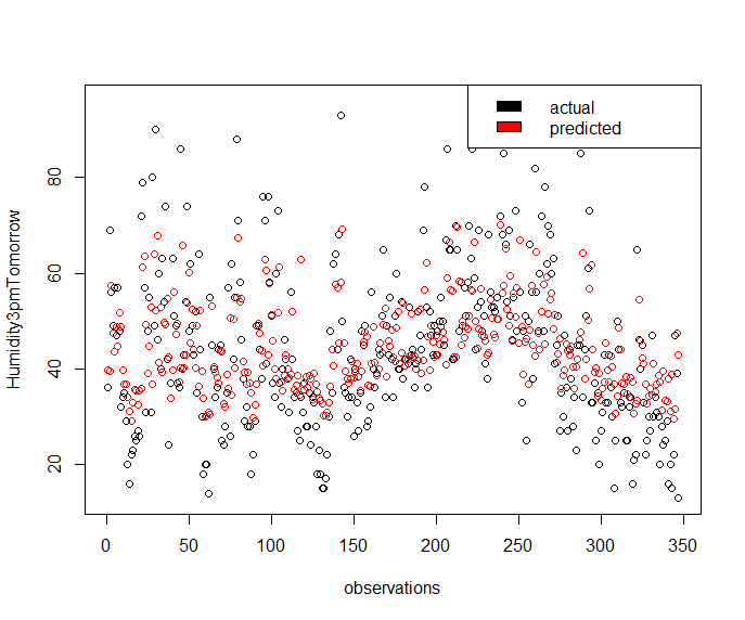
Tomorrow’s Humidity 3pm Prediction
h3pm_fit <- lm(Humidity3pmTomorrow ~ Humidity3pm + Sunshine, data = weather_data7)
summary(h3pm_fit)
Call:
lm(formula = Humidity3pmTomorrow ~ Humidity3pm + Sunshine, data = weather_data7)

Residuals:
    Min      1Q  Median      3Q     Max
-30.189  -9.117  -2.417   7.367  45.725

Coefficients:
            Estimate Std. Error t value Pr(>|t|)
(Intercept) 34.18668    5.45346   6.269 1.09e-09 ***
Humidity3pm  0.37697    0.06973   5.406 1.21e-07 ***
Sunshine    -0.85027    0.33476  -2.540   0.0115 *
---
Signif. codes:  0 ‘***’ 0.001 ‘**’ 0.01 ‘*’ 0.05 ‘.’ 0.1 ‘ ’ 1

Residual standard error: 14.26 on 344 degrees of freedom
Multiple R-squared:  0.2803,	Adjusted R-squared:  0.2761
F-statistic: 66.99 on 2 and 344 DF,  p-value: < 2.2e-16
All predictors are reported as significant.
lm_pred <- predict(h3pm_fit, weather_data7)
plot(x = seq_along(weather_data7$Humidity3pmTomorrow), y = weather_data7$Humidity3pmTomorrow, type='p', xlab = "observations", ylab = "Humidity3pmTomorrow")
legend("topright", c("actual", "predicted"), fill = c("black", "red"))
points(x = seq_along(weather_data7$Humidity3pmTomorrow), y = lm_pred, col='red')
Gives this plot.
Tomorrow’s WindGustSpeed Prediction
wgs_fit <- lm(WindGustSpeedTomorrow ~ WindGustSpeed + Pressure9am + Pressure3pm, data = weather_data7)
summary(wgs_fit)
Call:
lm(formula = WindGustSpeedTomorrow ~ Pressure9am + Pressure3pm +
    WindGustSpeed, data = weather_data7)

Residuals:
    Min      1Q  Median      3Q     Max
-31.252  -7.603  -1.069   6.155  49.984

Coefficients:
               Estimate Std. Error t value Pr(>|t|)
(Intercept)   620.53939  114.83812   5.404 1.22e-07 ***
Pressure9am     2.17983    0.36279   6.009 4.78e-09 ***
Pressure3pm    -2.76596    0.37222  -7.431 8.66e-13 ***
WindGustSpeed   0.23365    0.05574   4.192 3.52e-05 ***
---
Signif. codes:  0 ‘***’ 0.001 ‘**’ 0.01 ‘*’ 0.05 ‘.’ 0.1 ‘ ’ 1

Residual standard error: 11.29 on 343 degrees of freedom
Multiple R-squared:  0.2628,	Adjusted R-squared:  0.2563
F-statistic: 40.75 on 3 and 343 DF,  p-value: < 2.2e-16
All predictors are reported as significant.
lm_pred <- predict(wgs_fit, weather_data7)
plot(x = seq_along(weather_data7$WindGustSpeedTomorrow), y = weather_data7$WindGustSpeedTomorrow, type='p', xlab = "observations", ylab = "WindGustSpeedTomorrow")
legend("topright", c("actual", "predicted"), fill = c("black", "red"))
points(x = seq_along(weather_data7$WindGustSpeedTomorrow), y = lm_pred, col='red')
Gives this plot.

Tomorrow’s Sunshine Prediction
sun_fit <- lm(SunshineTomorrow ~ Sunshine*Humidity3pm + Cloud3pm + Evaporation + I(Evaporation^2) + WindGustSpeed - 1, data = weather_data7)
summary(sun_fit)
Call:
lm(formula = SunshineTomorrow ~ Sunshine * Humidity3pm + Cloud3pm +
    Evaporation + I(Evaporation^2) + WindGustSpeed - 1, data = weather_data7)

Residuals:
    Min      1Q  Median      3Q     Max
-9.9701 -1.8230  0.6534  2.1907  7.0478

Coefficients:
                      Estimate Std. Error t value Pr(>|t|)
Sunshine              0.607984   0.098351   6.182 1.82e-09 ***
Humidity3pm           0.062289   0.012307   5.061 6.84e-07 ***
Cloud3pm             -0.178190   0.082520  -2.159 0.031522 *
Evaporation           0.738127   0.245356   3.008 0.002822 **
I(Evaporation^2)     -0.050735   0.020510  -2.474 0.013862 *
WindGustSpeed         0.036675   0.013624   2.692 0.007453 **
Sunshine:Humidity3pm -0.007704   0.002260  -3.409 0.000729 ***
---
Signif. codes:  0 ‘***’ 0.001 ‘**’ 0.01 ‘*’ 0.05 ‘.’ 0.1 ‘ ’ 1

Residual standard error: 3.134 on 340 degrees of freedom
Multiple R-squared:  0.8718,	Adjusted R-squared:  0.8692
F-statistic: 330.3 on 7 and 340 DF,  p-value: < 2.2e-16
All predictors are reported as significant. Very good adjusted R-squared.
lm_pred <- predict(sun_fit, weather_data7)
plot(x = seq_along(weather_data7$SunshineTomorrow), y = weather_data7$SunshineTomorrow, type='p', xlab = "observations", ylab = "SunshineTomorrow")
legend("topright", c("actual", "predicted"), fill = c("black", "red"))
points(x = seq_along(weather_data7$SunshineTomorrow), y = lm_pred, col='red')
Gives this plot.
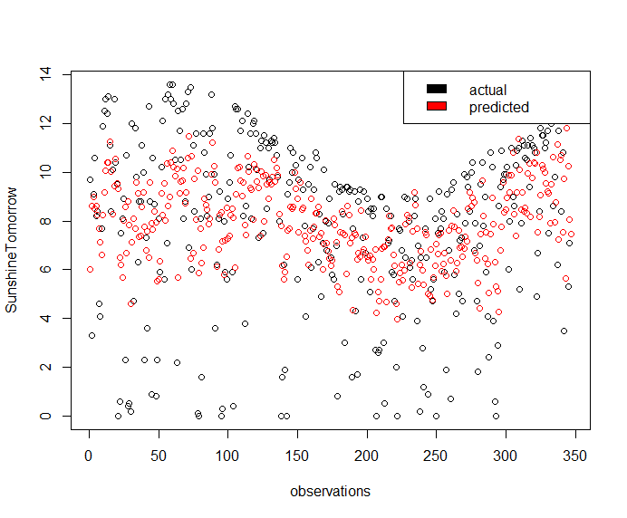
Above plot makes more evident that this model captures only a subset of the original Sunshine variance.
To give a more intuitive interpretation of the Sunshine information, it is suggestable to report a factor variable having levels:
{"Cloudy", "Mostly Cloudy", "Partly Cloudy", "Mostly Sunny", "Sunny"}
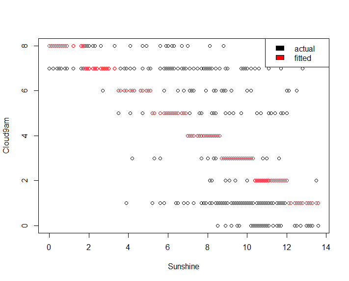
In doing that, we have furthermore to take into account tomorrow’s Cloud9am and Cloud3pm. For those quantitative variables, corresponding predictions are needed, and, at the purpose, the following linear regression models based on the Sunshine predictor can be depicted.
cloud9am_fit <- lm(Cloud9am ~ Sunshine, data = weather_data7)
summary(cloud9am_fit)
Call:
lm(formula = Cloud9am ~ Sunshine, data = weather_data7)

Residuals:
    Min      1Q  Median      3Q     Max
-5.2521 -1.7635 -0.4572  1.6920  5.9127

Coefficients:
            Estimate Std. Error t value Pr(>|t|)
(Intercept)  8.51527    0.28585   29.79   <2e-16 ***
Sunshine    -0.58031    0.03298  -17.59   <2e-16 ***
---
Signif. codes:  0 ‘***’ 0.001 ‘**’ 0.01 ‘*’ 0.05 ‘.’ 0.1 ‘ ’ 1

Residual standard error: 2.163 on 345 degrees of freedom
Multiple R-squared:  0.4729,	Adjusted R-squared:  0.4714
F-statistic: 309.6 on 1 and 345 DF,  p-value: < 2.2e-16
All predictors are reported as significant.
lm_pred <- round(predict(cloud9am_fit, weather_data7))
lm_pred[lm_pred == 9] = 8
plot(x = weather_data7$Sunshine, y = weather_data7$Cloud9am, type='p', xlab = "Sunshine", ylab = "Cloud9am")
legend("topright", c("actual", "predicted"), fill = c("black", "red"))
points(x = weather_data7$Sunshine, y = lm_pred, col='red')
Gives this plot.
cloud3pm_fit <- lm(Cloud3pm ~ Sunshine, data = weather_data7)
summary(cloud3pm_fit)
Call:
lm(formula = Cloud3pm ~ Sunshine, data = weather_data7)

Residuals:
    Min      1Q  Median      3Q     Max
-4.1895 -1.6230 -0.0543  1.4829  5.2883

Coefficients:
            Estimate Std. Error t value Pr(>|t|)
(Intercept)  8.01199    0.26382   30.37   <2e-16 ***
Sunshine    -0.50402    0.03044  -16.56   <2e-16 ***
---
Signif. codes:  0 ‘***’ 0.001 ‘**’ 0.01 ‘*’ 0.05 ‘.’ 0.1 ‘ ’ 1

Residual standard error: 1.996 on 345 degrees of freedom
Multiple R-squared:  0.4428,	Adjusted R-squared:  0.4412
F-statistic: 274.2 on 1 and 345 DF,  p-value: < 2.2e-16
All predictors are reported as significant.
lm_pred <- round(predict(cloud3pm_fit, weather_data7))
lm_pred[lm_pred == 9] = 8
plot(x = weather_data7$Sunshine, y = weather_data7$Cloud3pm, type='p', xlab = "Sunshine", ylab = "Cloud3pm")
legend("topright", c("actual", "predicted"), fill = c("black", "red"))
points(x = weather_data7$Sunshine, y = lm_pred, col='red')
Gives this plot.
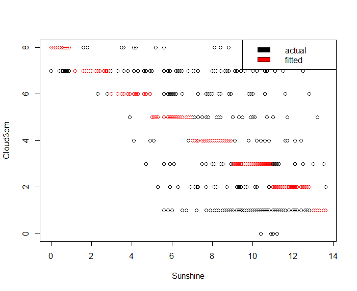
Once predicted the SunshineTomorrow value, we can use it as predictor input in Cloud9am/Cloud3pm linear regression models to determine both tomorrow’s Cloud9am and Cloud3pm predictions. We have preferred such approach in place of building a model based on one of the following formulas:
Cloud9amTomorrow ~ Cloud9am
Cloud9amTomorrow ~ Cloud9am + Sunshine
Cloud3pmTomorrow ~ Cloud3pm
because they provide with a very low adjusted R-squared (approximately in the interval [0.07, 0.08]).
Based on the Cloud9am and Cloud3pm predictions, the computation of a new factor variable named as CloudConditions and having levels {“Cloudy”, “Mostly Cloudy”, “Partly Cloudy”, “Mostly Sunny”, “Sunny”} will be shown. As we observed before our Sunshine prediction captures only a a subset of the variance of the modeled variable, and, as a consequence, our cloud conditions prediction is expected to rarely (possibly never) report “Cloudy” and “Sunny”.
Tomorrow’s MinTemp Prediction
minTemp_fit <- lm(MinTempTomorrow ~ MinTemp + Humidity3pm , data = weather_data7)
summary(minTemp_fit)
Call:
lm(formula = MinTempTomorrow ~ MinTemp + Humidity3pm, data = weather_data7)

Residuals:
     Min       1Q   Median       3Q      Max
-10.4820  -1.7546   0.3573   1.9119  10.0953

Coefficients:
             Estimate Std. Error t value Pr(>|t|)
(Intercept)  2.696230   0.520244   5.183 3.74e-07 ***
MinTemp      0.844813   0.027823  30.364  < 2e-16 ***
Humidity3pm -0.034404   0.009893  -3.478 0.000571 ***
---
Signif. codes:  0 ‘***’ 0.001 ‘**’ 0.01 ‘*’ 0.05 ‘.’ 0.1 ‘ ’ 1

Residual standard error: 3.112 on 344 degrees of freedom
Multiple R-squared:  0.7327,	Adjusted R-squared:  0.7311
F-statistic: 471.4 on 2 and 344 DF,  p-value: < 2.2e-16
All predictors are reported as significant.
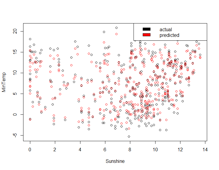
lm_pred <- predict(minTemp_fit, weather_data7)
plot(x = weather_data7$Sunshine, y = weather_data7$MinTemp, type='p', xlab = "Sunshine", ylab = "MinTemp")
legend("topright", c("actual", "fitted"), fill = c("black", "red"))
points(x = weather_data7$Sunshine, y = lm_pred, col='red')
Gives this plot.
Tomorrow’s MaxTemp Prediction
maxTemp_fit <- lm(MaxTempTomorrow ~ MaxTemp + Evaporation, data = weather_data7)
summary(maxTemp_fit)
Call:
lm(formula = MaxTempTomorrow ~ MaxTemp + Evaporation, data = weather_data7)

Residuals:
    Min      1Q  Median      3Q     Max
-13.217  -1.609   0.137   2.025   9.708

Coefficients:
            Estimate Std. Error t value Pr(>|t|)
(Intercept)  2.69811    0.56818   4.749 3.01e-06 ***
MaxTemp      0.82820    0.03545  23.363  < 2e-16 ***
Evaporation  0.20253    0.08917   2.271   0.0237 *
---
Signif. codes:  0 ‘***’ 0.001 ‘**’ 0.01 ‘*’ 0.05 ‘.’ 0.1 ‘ ’ 1

Residual standard error: 3.231 on 344 degrees of freedom
Multiple R-squared:  0.7731,	Adjusted R-squared:  0.7718
F-statistic:   586 on 2 and 344 DF,  p-value: < 2.2e-16
All predictors are reported as significant.
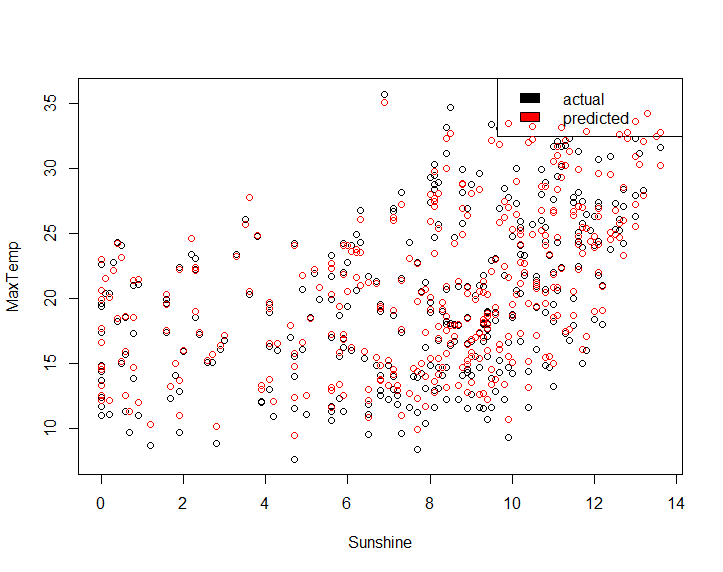
lm_pred <- predict(maxTemp_fit, weather_data7)
plot(x = weather_data7$Sunshine, y = weather_data7$MaxTemp, type='p', xlab = "Sunshine", ylab = "MaxTemp")
legend("topright", c("actual", "fitted"), fill = c("black", "red"))
points(x = weather_data7$Sunshine, y = lm_pred, col='red')
Gives this plot.
CloudConditions computation
Based on second reference given at the end, we have the following mapping between a descriptive cloud conditions string and the cloud coverage in ”oktas,” which are a unit of eights.
Cloudy: 8/8 opaque clouds
Mostly Cloudy: 6/8 - 7/8 opaque clouds
Partly Cloudy: 3/8 - 5/8 opaque clouds
Mostly Sunny: 1/8 - 2/8 opaque clouds
Sunny: 0/8 opaque clouds
We can figure out the following utility function to help.
computeCloudConditions = function(cloud_9am, cloud_3pm) {
   cloud_avg = min(round((cloud_9am + cloud_3pm)/2), 8)
   cc_str = NULL
   if (cloud_avg == 8) {
     cc_str = "Cloudy"
   } else if (cloud_avg >= 6) {
     cc_str = "Mostly Cloudy"
   } else if (cloud_avg >= 3) {
     cc_str = "Partly Cloudy"
   } else if (cloud_avg >= 1) {
     cc_str = "Mostly Sunny"
   } else if (cloud_avg < 1) {
     cc_str = "Sunny"
   }
   cc_str
}
Weather Forecast Report
Starting from a basic example of weather dataset, we were able to build several regression models. The first one, based on logistic regression, is capable of predict the RainTomorrow factor variable. The linear regression models are to predict the Rainfall, Humidity3pm, WindGustSpeed, MinTemp, MaxTemp, CloudConditions weather metrics. The overall picture we got is the following.
                                +----------------+
                                |                |
                                |                +------> RainTomorrow
                                |                |
                                |   Weather      +------> Rainfall
                                |                |
{Today's weather data} ---->----+   Forecast     +------> Humidity3pm
                                |                |
                                |   Models       +------> WindGustSpeed          +-----------------------+
                                |                |                               | linear regression     |
                                |                +------> Sunshine ------>-------+       models          +-->--{Cloud9am, Cloud3pm}--+
                                |                |                               | Cloud9am and Cloud3pm |                           |
                                |                +------> MinTemp                +-----------------------+                           |
                                |                |                                                                                   |
                                |                +------> MaxTemp                                                                    |
                                |                |                                                                                   |
                                +----------------+                               +-----------------------+                           |
                                                                                 |    computing new      |                           |
              { Cloudy, Mostly Cloudy, Partly Cloudy, Mostly Sunny, Sunny} <-----+    factor variable    +-------------<-------------+
                                                                                 |    CloudConditions    |
                                                                                 +-----------------------+
As said before, if RainTomorrow == “Yes” Rainfall is explicitely given, otherwise un upper bound Rainfall < 1 mm is. Chance of rain is computed only if RainTomorrow prediction is “Yes”. The Humidity3pm prediction is taken as humidity prediction for the whole day, in general.
weather_report <- function(today_record, rain_tomorrow_model, cutoff) {
    # RainTomorrow  prediction
    rainTomorrow_prob <- predict(rain_tomorrow_model, today_record, type="prob")
    rainTomorrow_pred = ifelse(rainTomorrow_prob$Yes >= cutoff, "Yes", "No")

    # Rainfall prediction iff RainTomorrow prediction is Yes; chance of rain probability
    rainfall_pred <- NA
    chance_of_rain <- NA
    if (rainTomorrow_pred == "Yes") {
        rainfall_pred <- round(predict(rf_fit, today_record), 1)
        chance_of_rain <- round(rainTomorrow_prob$Yes*100)
    }

    # WindGustSpeed prediction
    wgs_pred <- round(predict(wgs_fit, today_record), 1)

    # Humidity3pm prediction
    h3pm_pred <- round(predict(h3pm_fit, today_record), 1)

    # sunshine prediction is used to fit Cloud9am and Cloud3pm
    sun_pred <- predict(sun_fit, today_record)

    cloud9am_pred <- min(round(predict(cloud9am_fit, data.frame(Sunshine=sun_pred))), 8)
    cloud3pm_pred <- min(round(predict(cloud3pm_fit, data.frame(Sunshine=sun_pred))), 8)
    # a descriptive cloud conditions string is computed
    CloudConditions_pred <- computeCloudConditions(cloud9am_pred, cloud3pm_pred)

    # MinTemp prediction
    minTemp_pred <- round(predict(minTemp_fit, today_record), 1)

    # MaxTemp prediction
    maxTemp_pred <- round(predict(maxTemp_fit, today_record), 1)

    # converting all numeric predictions to strings
    if (is.na(rainfall_pred)) {
      rainfall_pred_str <- "< 1 mm"
    } else {
      rainfall_pred_str <- paste(rainfall_pred, "mm", sep = " ")
    }

    if (is.na(chance_of_rain)) {
      chance_of_rain_str <- ""
    } else {
      chance_of_rain_str <- paste(chance_of_rain, "%", sep="")
    }

    wgs_pred_str <- paste(wgs_pred, "Km/h", sep= " ")
    h3pm_pred_str <- paste(h3pm_pred, "%", sep = "")
    minTemp_pred_str <- paste(minTemp_pred, "°C", sep= "")
    maxTemp_pred_str <- paste(maxTemp_pred, "°C", sep= "")

    report <- data.frame(Rainfall = rainfall_pred_str,
                      ChanceOfRain = chance_of_rain_str,
                      WindGustSpeed = wgs_pred_str,
                      Humidity = h3pm_pred_str,
                      CloudConditions = CloudConditions_pred,
                      MinTemp = minTemp_pred_str,
                      MaxTemp = maxTemp_pred_str)
   report
}
Sure there are confidence and prediction intervals associated to our predictions. However, since we intend to report our forecasts to Canberra’s citizens, our message should be put in simple words to reach everybody and not just statisticians.
Finally we can try our tomorrow weather forecast report out.
(tomorrow_report <- weather_report(weather_data[10,], mod_ev_c3_fit, 0.56))
Rainfall ChanceOfRain WindGustSpeed Humidity CloudConditions MinTemp MaxTemp
1   < 1 mm                  36.9 Km/h    39.7%   Partly Cloudy  8.7°C  22.7°C
(tomorrow_report <- weather_report(weather_data[32,], mod_ev_c3_fit, 0.56))
Rainfall ChanceOfRain WindGustSpeed Humidity CloudConditions MinTemp MaxTemp
1   < 1 mm                    48 Km/h    41.3%   Partly Cloudy  10.9°C  24.8°C
(tomorrow_report <- weather_report(weather_data[50,], mod_ev_c3_fit, 0.56))
Rainfall ChanceOfRain WindGustSpeed Humidity CloudConditions MinTemp MaxTemp
1   8.3 mm          59%     36.9 Km/h    60.1%   Partly Cloudy  10.8°C  22.2°C
(tomorrow_report <- weather_report(weather_data[100,], mod_ev_c3_fit, 0.56))
Rainfall ChanceOfRain WindGustSpeed Humidity CloudConditions MinTemp MaxTemp
1   5.4 mm          71%     46.7 Km/h    51.3%   Partly Cloudy  11.2°C  20.3°C
(tomorrow_report <- weather_report(weather_data[115,], mod_ev_c3_fit, 0.56))
Rainfall ChanceOfRain WindGustSpeed Humidity CloudConditions MinTemp MaxTemp
1   < 1 mm                  46.4 Km/h    35.7%    Mostly Sunny  12.3°C  25.1°C
(tomorrow_report <- weather_report(weather_data[253,], mod_ev_c3_fit, 0.56))
Rainfall ChanceOfRain WindGustSpeed Humidity CloudConditions MinTemp MaxTemp
1   9.4 mm          81%     52.4 Km/h    65.2%   Partly Cloudy   1.3°C  10.3°C
(tomorrow_report <- weather_report(weather_data[311,], mod_ev_c3_fit, 0.56))
Rainfall ChanceOfRain WindGustSpeed Humidity CloudConditions MinTemp MaxTemp
1   < 1 mm                  40.7 Km/h    44.2%   Mostly Cloudy   6.9°C  16.4°C
Please note that some records of the original weather dataset may show NA’s values and our regression models did not cover a predictor can be as such. To definitely evaluate the accuracy of our weather forecast report, we would need to check its unseen data predictions with the occurred tomorrow’s weather. Further, to improve the adjusted R-squared metric of our linear regression models is a potential area of investigation.
Conclusions
Starting from a basic weather dataset, we went through an interesting datastory involving exploratory analysis and models building. We spot strengths and weaknesses of our prediction models. We also learned some insights of the meteorology terminology.
We hope you enjoyed this tutorial series on weather forecast. If you have any questions, please feel free to comment below.
References