In this tutorial we are going to analyse a weather dataset to produce exploratory analysis and forecast reports based on regression models.
We are going to explore a public dataset which is part of the exercise datasets of the “Data Mining and Business Analytics with R” book (Wiley) written by Johannes Ledolter. In doing that, we are taking advantage of several R packages, caret package included.
The tutorial is going to be split in the following four parts:
-
1. Introducing the weather dataset and outlining its exploratory analysis
2. Building logistic regression models for 9am, 3pm and late evening weather forecasts
3. Tuning to improve accuracy of previously build models and show ROC plots
4. Making considerations on “at-least” moderate rainfall scenarios and building additional models to predict further weather variables
R Packages
Overall, we are going to make use of the following packages:
suppressPackageStartupMessages(library(knitr))
suppressPackageStartupMessages(library(caret))
suppressPackageStartupMessages(library(gmodels))
suppressPackageStartupMessages(library(lattice))
suppressPackageStartupMessages(library(ggplot2))
suppressPackageStartupMessages(library(gridExtra))
suppressPackageStartupMessages(library(Kmisc))
suppressPackageStartupMessages(library(ROCR))
suppressPackageStartupMessages(library(corrplot))
Exploratory Analysis
The dataset under analysis is publicly available at:
jledolter – datamining – data exercises
It contains daily observations from a single weather station. Let us start by loading the data and taking a look at.
set.seed(1023)
weather_data <- read.csv(url("https://www.biz.uiowa.edu/faculty/jledolter/datamining/weather.csv"), header = TRUE, sep = ",", stringsAsFactors = TRUE)
kable(head(weather_data))
|Date      |Location | MinTemp| MaxTemp| Rainfall| Evaporation| Sunshine|WindGustDir | WindGustSpeed|WindDir9am |WindDir3pm | WindSpeed9am| WindSpeed3pm| Humidity9am| Humidity3pm| Pressure9am| Pressure3pm| Cloud9am| Cloud3pm| Temp9am| Temp3pm|RainToday | RISK_MM|RainTomorrow |
|:---------|:--------|-------:|-------:|--------:|-----------:|--------:|:-----------|-------------:|:----------|:----------|------------:|------------:|-----------:|-----------:|-----------:|-----------:|--------:|--------:|-------:|-------:|:---------|-------:|:------------|
|11/1/2007 |Canberra |     8.0|    24.3|      0.0|         3.4|      6.3|NW          |            30|SW         |NW         |            6|           20|          68|          29|      1019.7|      1015.0|        7|        7|    14.4|    23.6|No        |     3.6|Yes          |
|11/2/2007 |Canberra |    14.0|    26.9|      3.6|         4.4|      9.7|ENE         |            39|E          |W          |            4|           17|          80|          36|      1012.4|      1008.4|        5|        3|    17.5|    25.7|Yes       |     3.6|Yes          |
|11/3/2007 |Canberra |    13.7|    23.4|      3.6|         5.8|      3.3|NW          |            85|N          |NNE        |            6|            6|          82|          69|      1009.5|      1007.2|        8|        7|    15.4|    20.2|Yes       |    39.8|Yes          |
|11/4/2007 |Canberra |    13.3|    15.5|     39.8|         7.2|      9.1|NW          |            54|WNW        |W          |           30|           24|          62|          56|      1005.5|      1007.0|        2|        7|    13.5|    14.1|Yes       |     2.8|Yes          |
|11/5/2007 |Canberra |     7.6|    16.1|      2.8|         5.6|     10.6|SSE         |            50|SSE        |ESE        |           20|           28|          68|          49|      1018.3|      1018.5|        7|        7|    11.1|    15.4|Yes       |     0.0|No           |
|11/6/2007 |Canberra |     6.2|    16.9|      0.0|         5.8|      8.2|SE          |            44|SE         |E          |           20|           24|          70|          57|      1023.8|      1021.7|        7|        5|    10.9|    14.8|No        |     0.2|No           |
Metrics at specific Date and Location are given together with the RainTomorrow variable indicating if rain occurred on next day.
colnames(weather_data)
[1] "Date"          "Location"      "MinTemp"       "MaxTemp"       "Rainfall"
[6] "Evaporation"   "Sunshine"      "WindGustDir"   "WindGustSpeed" "WindDir9am"
[11] "WindDir3pm"    "WindSpeed9am"  "WindSpeed3pm"  "Humidity9am"   "Humidity3pm"
[16] "Pressure9am"   "Pressure3pm"   "Cloud9am"      "Cloud3pm"      "Temp9am"
[21] "Temp3pm"       "RainToday"     "RISK_MM"       "RainTomorrow"
The description of the variables is the following.
-
Date: The date of observation (a date object).
Location: The common name of the location of the weather station
MinTemp: The minimum temperature in degrees centigrade
MaxTemp: The maximum temperature in degrees centigrade
Rainfall: The amount of rainfall recorded for the day in millimeters.
Evaporation: Class A pan evaporation (in millimeters) during 24 h
Sunshine: The number of hours of bright sunshine in the day
WindGustDir: The direction of the strongest wind gust in the 24 h to midnight
WindGustSpeed: The speed (in kilometers per hour) of the strongest wind gust in the 24 h to midnight
WindDir9am: The direction of the wind gust at 9 a.m.
WindDir3pm: The direction of the wind gust at 3 p.m.
WindSpeed9am: Wind speed (in kilometers per hour) averaged over 10 min before 9 a.m.
WindSpeed3pm: Wind speed (in kilometers per hour) averaged over 10 min before 3 p.m.
Humidity9am: Relative humidity (in percent) at 9 am
Humidity3pm: Relative humidity (in percent) at 3 pm
Pressure9am: Atmospheric pressure (hpa) reduced to mean sea level at 9 a.m.
Pressure3pm: Atmospheric pressure (hpa) reduced to mean sea level at 3 p.m.
Cloud9am: Fraction of sky obscured by cloud at 9 a.m. This is measured in ”oktas,” which are a unit of eighths. It records how many eighths of the sky are obscured by cloud. A 0 measure indicates completely clear sky, while an 8 indicates that it is completely overcast
Cloud3pm: Fraction of sky obscured by cloud at 3 p.m; see Cloud9am for a description of the values
Temp9am: Temperature (degrees C) at 9 a.m.
Temp3pm: Temperature (degrees C) at 3 p.m.
RainToday: Integer 1 if precipitation (in millimeters) in the 24 h to 9 a.m. exceeds 1 mm, otherwise 0
RISK_MM: The continuous target variable; the amount of rain recorded during the next day
RainTomorrow: The binary target variable whether it rains or not during the next day
Looking then at the data structure, we discover the dataset includes a mix of numerical and categorical variables.
str(weather_data)
> str(weather_data)
'data.frame':	366 obs. of  24 variables:
 $ Date         : Factor w/ 366 levels "1/1/2008","1/10/2008",..: 63 74 85 87 88 89 90 91 92 64 ...
 $ Location     : Factor w/ 1 level "Canberra": 1 1 1 1 1 1 1 1 1 1 ...
 $ MinTemp      : num  8 14 13.7 13.3 7.6 6.2 6.1 8.3 8.8 8.4 ...
 $ MaxTemp      : num  24.3 26.9 23.4 15.5 16.1 16.9 18.2 17 19.5 22.8 ...
 $ Rainfall     : num  0 3.6 3.6 39.8 2.8 0 0.2 0 0 16.2 ...
 $ Evaporation  : num  3.4 4.4 5.8 7.2 5.6 5.8 4.2 5.6 4 5.4 ...
 $ Sunshine     : num  6.3 9.7 3.3 9.1 10.6 8.2 8.4 4.6 4.1 7.7 ...
 $ WindGustDir  : Factor w/ 16 levels "E","ENE","ESE",..: 8 2 8 8 11 10 10 1 9 1 ...
 $ WindGustSpeed: int  30 39 85 54 50 44 43 41 48 31 ...
 $ WindDir9am   : Factor w/ 16 levels "E","ENE","ESE",..: 13 1 4 15 11 10 10 10 1 9 ...
 $ WindDir3pm   : Factor w/ 16 levels "E","ENE","ESE",..: 8 14 6 14 3 1 3 1 2 3 ...
 $ WindSpeed9am : int  6 4 6 30 20 20 19 11 19 7 ...
 $ WindSpeed3pm : int  20 17 6 24 28 24 26 24 17 6 ...
 $ Humidity9am  : int  68 80 82 62 68 70 63 65 70 82 ...
 $ Humidity3pm  : int  29 36 69 56 49 57 47 57 48 32 ...
 $ Pressure9am  : num  1020 1012 1010 1006 1018 ...
 $ Pressure3pm  : num  1015 1008 1007 1007 1018 ...
 $ Cloud9am     : int  7 5 8 2 7 7 4 6 7 7 ...
 $ Cloud3pm     : int  7 3 7 7 7 5 6 7 7 1 ...
 $ Temp9am      : num  14.4 17.5 15.4 13.5 11.1 10.9 12.4 12.1 14.1 13.3 ...
 $ Temp3pm      : num  23.6 25.7 20.2 14.1 15.4 14.8 17.3 15.5 18.9 21.7 ...
 $ RainToday    : Factor w/ 2 levels "No","Yes": 1 2 2 2 2 1 1 1 1 2 ...
 $ RISK_MM      : num  3.6 3.6 39.8 2.8 0 0.2 0 0 16.2 0 ...
 $ RainTomorrow : Factor w/ 2 levels "No","Yes": 2 2 2 2 1 1 1 1 2 1 ...
We have available 366 records:
(n <- nrow(weather_data))
[1] 366
which spans the following timeline:
c(as.character(weather_data$Date[1]), as.character(weather_data$Date[n]))
[1] "11/1/2007"  "10/31/2008"
We further notice that RISK_MM relation with the RainTomorrow variable is the following.
all.equal(weather_data$RISK_MM > 1, weather_data$RainTomorrow == "Yes")
[1] TRUE
The Rainfall variable and the RainToday are equivalent according to the following relationship (as anticipated by the Rainfall description).
all.equal(weather_data$Rainfall > 1, weather_data$RainToday == "Yes")
[1] TRUE
To make it more challenging, we decide to take RISK_MM, RainFall and RainToday out, and determine a new dataset as herein depicted.
weather_data2 <- subset(weather_data, select = -c(Date, Location, RISK_MM, Rainfall, RainToday))
colnames(weather_data2)
[1] "MinTemp"       "MaxTemp"       "Evaporation"   "Sunshine"      "WindGustDir"   "WindGustSpeed"
[7] "WindDir9am"    "WindDir3pm"    "WindSpeed9am"  "WindSpeed3pm"  "Humidity9am"   "Humidity3pm"
[13] "Pressure9am"   "Pressure3pm"   "Cloud9am"      "Cloud3pm"      "Temp9am"       "Temp3pm"
[19] "RainTomorrow"
(cols_withNa <- apply(weather_data2, 2, function(x) sum(is.na(x))))
MinTemp       MaxTemp   Evaporation      Sunshine   WindGustDir WindGustSpeed    WindDir9am
            0             0             0             3             3             2            31
   WindDir3pm  WindSpeed9am  WindSpeed3pm   Humidity9am   Humidity3pm   Pressure9am   Pressure3pm
            1             7             0             0             0             0             0
     Cloud9am      Cloud3pm       Temp9am       Temp3pm  RainTomorrow
            0             0             0             0             0
Look at the NA’s counts associated to WindDir9am. If WindDir9am were a not significative predictor for RainTomorrow, we could take such data column out and increased the complete cases count. When dealing with the categorical variable analysis we determine if that is possible. For now, we consider records without NA’s values.
weather_data3 <- weather_data2[complete.cases(weather_data2),]
Categorical Variable Analysis
factor_vars <- names(which(sapply(weather_data3, class) == "factor"))
factor_vars <- setdiff(factor_vars, "RainTomorrow")
chisq_test_res <- lapply(factor_vars, function(x) {
  chisq.test(weather_data3[,x], weather_data3[, "RainTomorrow"], simulate.p.value = TRUE)
  })
names(chisq_test_res) <- factor_vars
chisq_test_res
$WindGustDir

	Pearson's Chi-squared test with simulated p-value (based on 2000 replicates)

data:  weather_data3[, x] and weather_data3[, "RainTomorrow"]
X-squared = 35.833, df = NA, p-value = 0.001999

$WindDir9am

	Pearson's Chi-squared test with simulated p-value (based on 2000 replicates)

data:  weather_data3[, x] and weather_data3[, "RainTomorrow"]
X-squared = 23.813, df = NA, p-value = 0.06547

$WindDir3pm

	Pearson's Chi-squared test with simulated p-value (based on 2000 replicates)

data:  weather_data3[, x] and weather_data3[, "RainTomorrow"]
X-squared = 9.403, df = NA, p-value = 0.8636
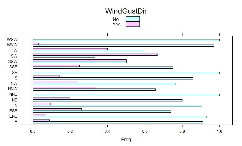
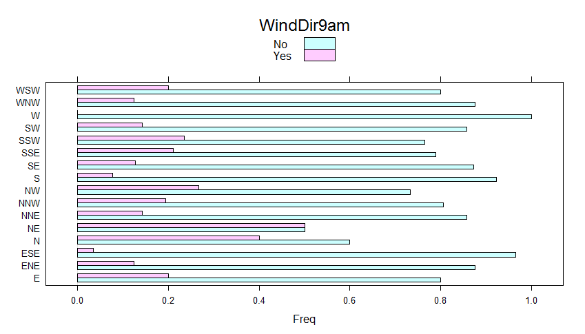
Above shown Chi-squared p-value results tell us that RainTomorrow values depend upon WindGustDir (we reject the null hypothesis that RainTomorrow does not depend upon the WindGustDir). We do not reject the null-hypothesis for WindDir9am and WindDir3pm as p.value > 0.05, hence RainTomorrow does not depend upon those two predictors. We, therefore, expect to take advantage of WindGustDir as a predictor and not to consider WindDir9am and WindDir3pm for such purpose.
It is also possible to obtain a visual understanding of the significance of such categorical variables by taking advantage of bar charts with the cross table row proportions as input.
barchart_res <- lapply(factor_vars, function(x) {
  title <- colnames(weather_data3[,x, drop=FALSE])
  wgd <- CrossTable(weather_data3[,x], weather_data3$RainTomorrow, prop.chisq=F)
  barchart(wgd$prop.row, stack=F, auto.key=list(rectangles = TRUE, space = "top", title = title))
})
names(barchart_res) <- factor_vars
barchart_res$WindGustDir
Barchart of WindGustDir
barchart_res$WindDir9am
Barchart of WindDir9am
barchart_res$WindDir3pm
Barchart of WindDir3pm
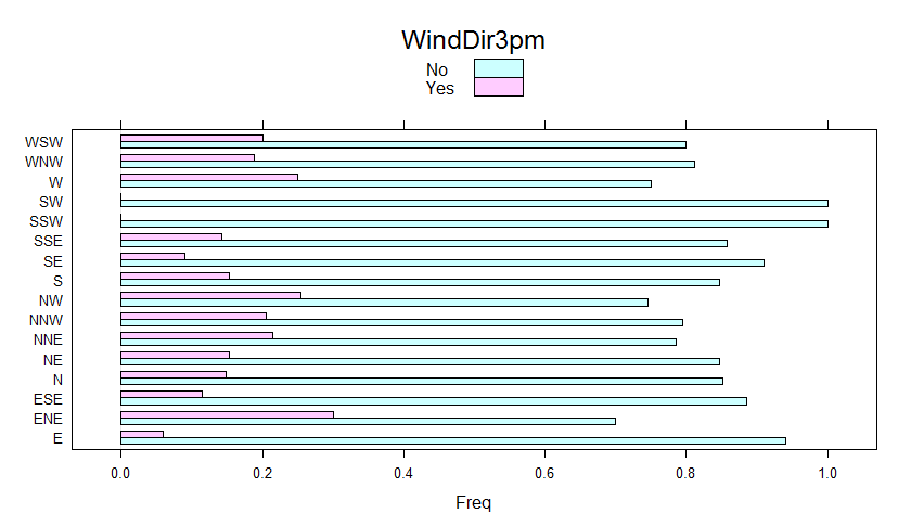
Being WindDir9am not a candidate predictor and having got more than 30 NA’s values, we decide to take it out. As a consequence, we have increased the number of NA-free records from 328 to 352. Same for WindDir3pm.
weather_data4 <- subset(weather_data2, select = -c(WindDir9am, WindDir3pm))
weather_data5 <- weather_data4[complete.cases(weather_data4),]
colnames(weather_data5)
[1] "MinTemp"       "MaxTemp"       "Evaporation"   "Sunshine"      "WindGustDir"
 [6] "WindGustSpeed" "WindSpeed9am"  "WindSpeed3pm"  "Humidity9am"   "Humidity3pm"
[11] "Pressure9am"   "Pressure3pm"   "Cloud9am"      "Cloud3pm"      "Temp9am"
[16] "Temp3pm"       "RainTomorrow"
So, we end up with a dataset made up of 16 potential predictors, one of those is a categorical variable (WindGustDir) and 15 are quantitative.
Quantitative Variable Analysis
In this section, we carry on the exploratory analysis of quantitative variables. We start first by a visualization of the correlation relationship among variables.
factor_vars <- names(which(sapply(weather_data5, class) == "factor"))
numeric_vars <- setdiff(colnames(weather_data5), factor_vars)
numeric_vars <- setdiff(numeric_vars, "RainTomorrow")
numeric_vars
numeric_vars_mat <- as.matrix(weather_data5[, numeric_vars, drop=FALSE])
numeric_vars_cor <- cor(numeric_vars_mat)
corrplot(numeric_vars_cor)
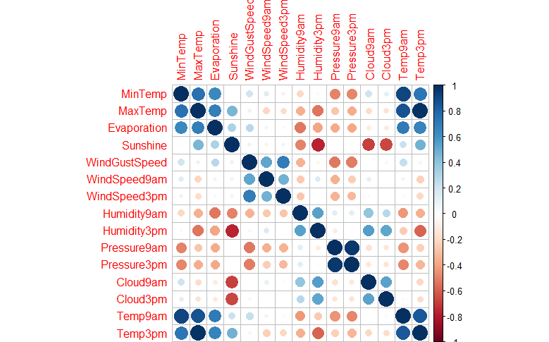
By taking a look at above shown correlation plot, we can state that:
- Temp9am strongly positive correlated with MinTemp
- Temp9am strongly positive correlated with MaxTemp
- Temp9am strongly positive correlated with Temp3pm
- Temp3pm strongly positive correlated with MaxTemp
- Pressure9am strongly positive correlated with Pressure3pm
- Humidity3pm strongly negative correlated with Sunshine
- Cloud9am strongly negative correlated with Sunshine
- Cloud3pm strongly negative correlated with Sunshine
The pairs plot put in evidence if any relationship among variables is in place, such as a linear relationship.
pairs(weather_data5[,numeric_vars], col=weather_data5$RainTomorrow)
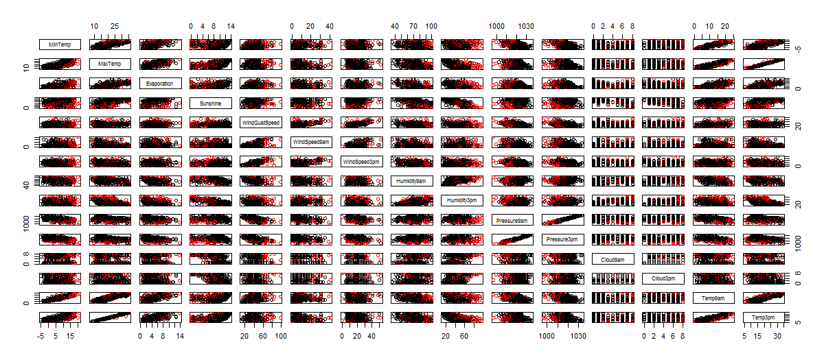
Visual analysis, put in evidence a linear relationship among the following variable pairs:
- MinTemp and MaxTemp
- MinTemp and Evaporation
- MaxTemp and Evaporation
- Temp9am and MinTemp
- Temp3pm and MaxTemp
- Pressure9am and Pressure3pm
- Humidity9am and Humidity3pm
- WindSpeed9am and WindGustSpeed
- WindSpeed3pm and WindGustSpeed
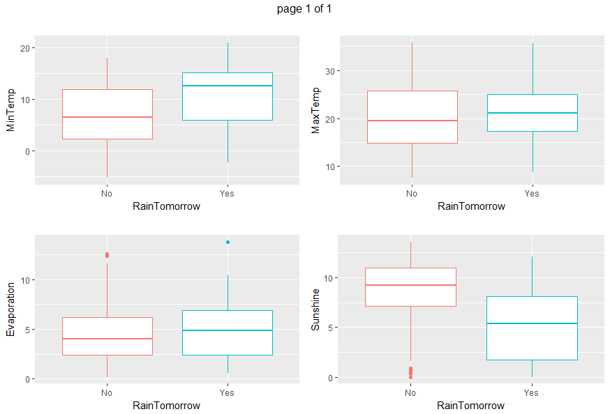
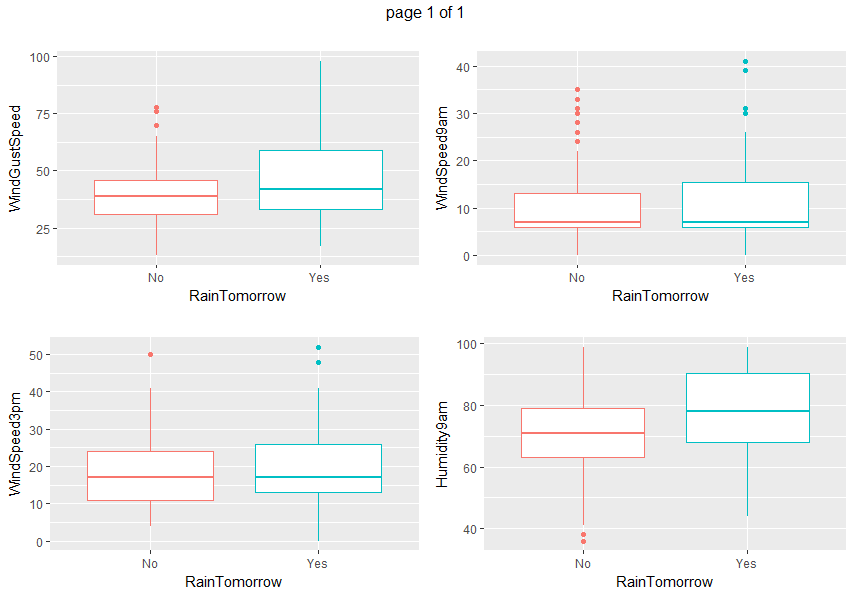
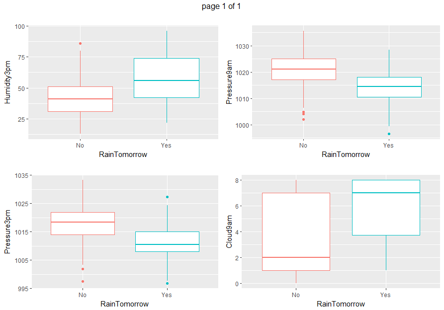
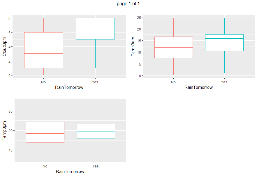
Boxplots and density plots give a visual understanding of the significance of a predictor by looking at how much are overlapping the predictor values set depending on the variable to be predicted (RainTomorrow).
gp <- invisible(lapply(numeric_vars, function(x) {
  ggplot(data=weather_data5, aes(x= RainTomorrow, y=eval(parse(text=x)), col = RainTomorrow)) + geom_boxplot() + xlab("RainTomorrow") + ylab(x) + ggtitle("") + theme(legend.position="none")}))
grob_plots <- invisible(lapply(chunk(1, length(gp), 4), function(x) {
  marrangeGrob(grobs=lapply(gp[x], ggplotGrob), nrow=2, ncol=2)}))
grob_plots
gp <- invisible(lapply(numeric_vars, function(x) {
  ggplot(data=weather_data5, aes(x=eval(parse(text=x)), col = RainTomorrow)) + geom_density() + xlab(x) + ggtitle(paste(x, "density", sep= " "))}))
grob_plots <- invisible(lapply(chunk(1, length(gp), 4), function(x) {
  marrangeGrob(grobs=lapply(gp[x], ggplotGrob), nrow=2, ncol=2)}))
grob_plots
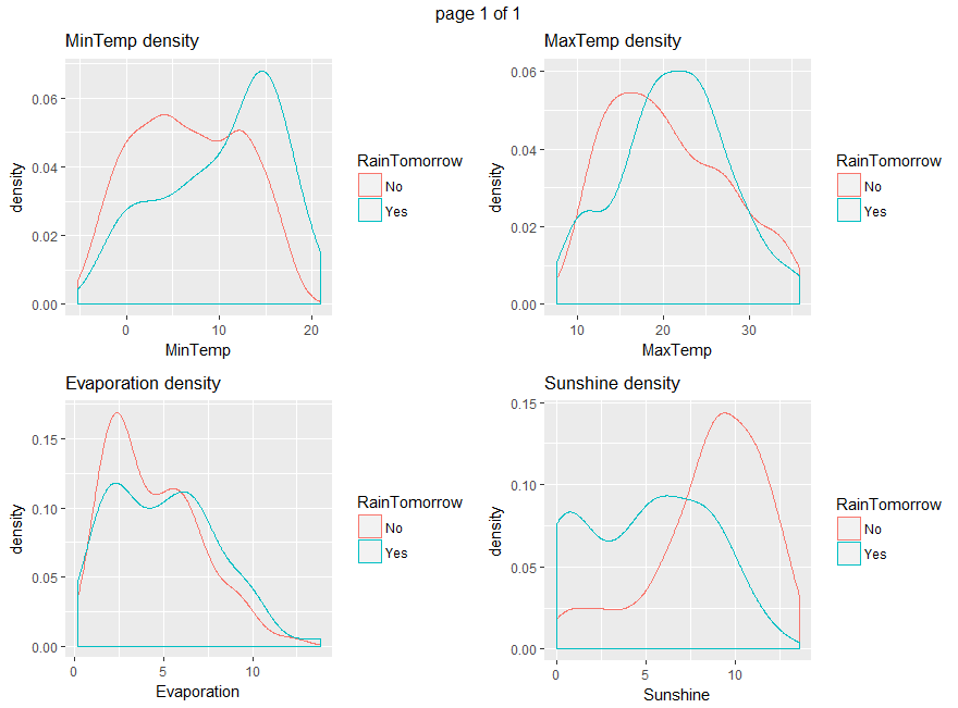
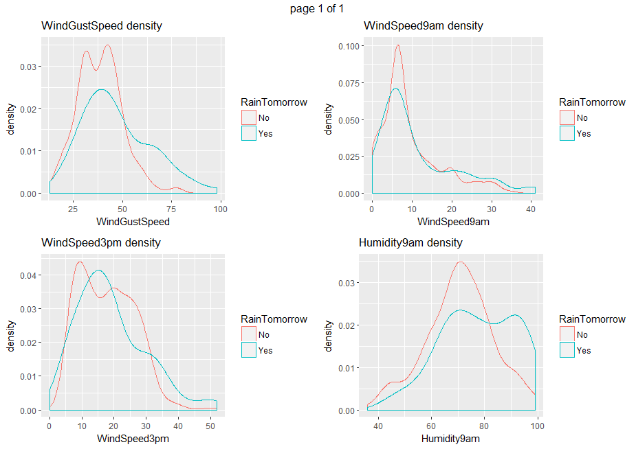
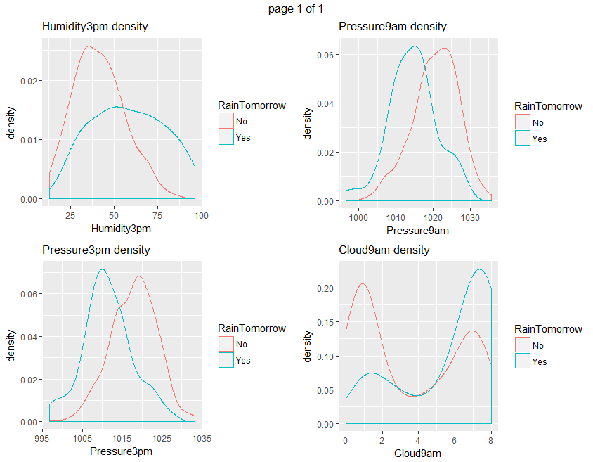

From all those plots, we can state that Humidity3pm, Pressure9am, Pressure3pm, Cloud9am, Cloud3pm and Sunshine are predictors to be considered.
Ultimately, we save the dataset currently under analysis for the prosecution of this tutorial.
write.csv(weather_data5, file="weather_data5.csv", sep=",", row.names=FALSE)
Conclusions
Exploratory analysis has highlighted interesting relationships across variables. Such preliminary results give us hints for predictors selection and will be considered in the prosecution of this analysis.
If you have any questions, please feel free to comment below.
References
-
Data Mining and Business Analytics with R, Johannes Ledolter, Wiley