Visualizing Streaming Data And Alert Notification with Shiny

Streaming Data is data that is generated continuously and it includes various sources such as sensors, log files, geospatial services, etc. The data may come at regular intervals and we may want to have a dashboard which updates by itself and incorporates the newly added data so that we can use it for deta driven decision making. For example in IOT, it can help to monitor sensors which are failing or sensors which report abnormal readings.

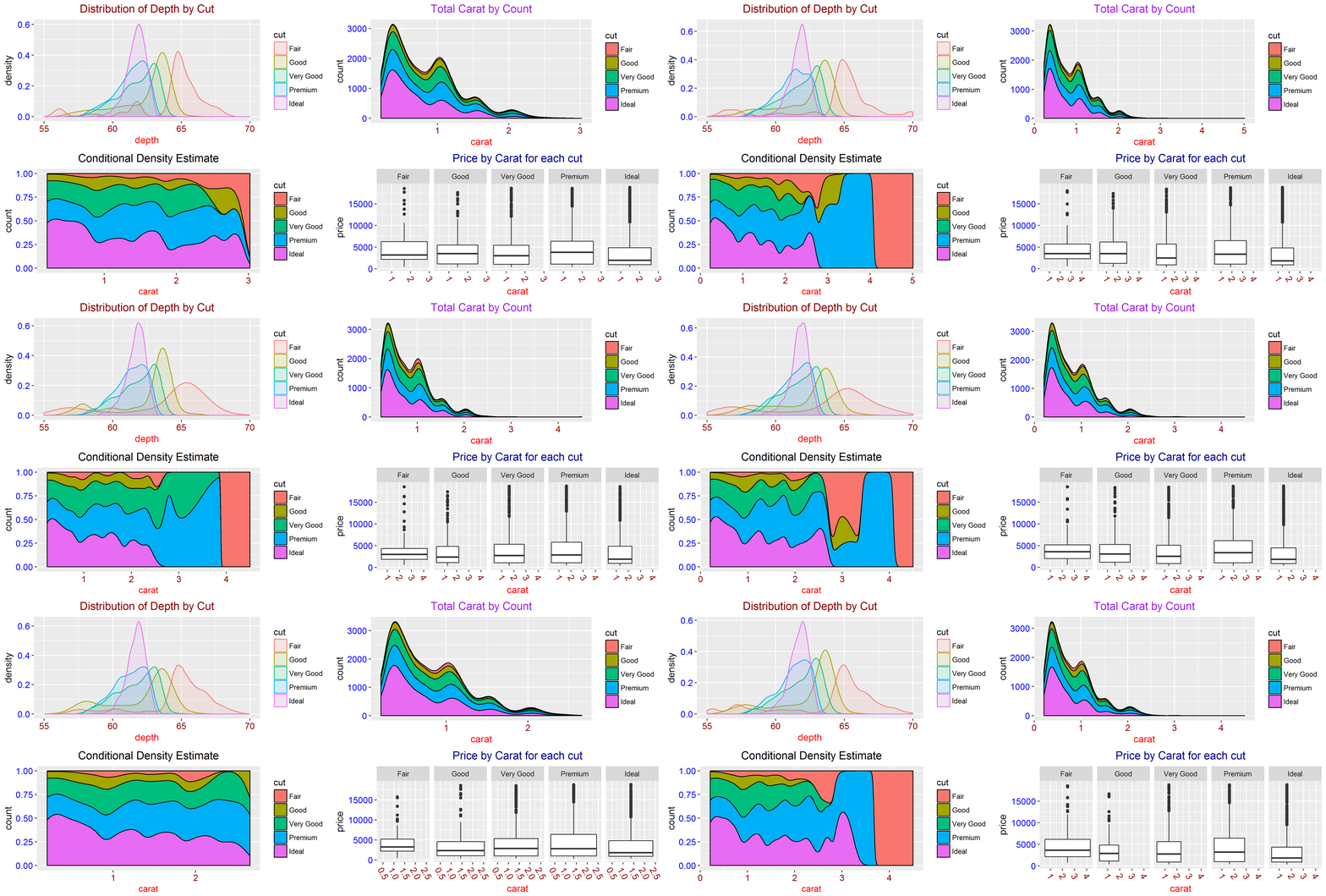
This week short blog post is on visualizing streaming data using shiny. The dashboard updates automatically to incorporate newly added data. In the end of this post you will find a video tutorial on how to send text and email alerts, based on streaming sensor data, when there is an abnormal reading or when a sensor fails.

library(ggplot2)
library(dplyr)
data("diamonds")

while(TRUE){
        temp=sample_frac(diamonds,0.1)
        write.csv(temp, paste0("sampled", gsub("[^0-9]","",Sys.time()),".csv"),
                  row.names = FALSE)
        Sys.sleep(10) # Suspend execution of R expressions. The time interval to suspend execution for, in seconds.

}

Then, the following are the shiny code that fetch the newly generated data and create a shiny dashboard.

ui.R

library(shiny)
fluidPage(
        tags$h2("Visualizing Streaming Data with Shiny",
                style="color:blue;text-align:center"),
        plotOutput("plot1",height = "600px")
     )

server.R

library(shiny)
library(data.table)
library(ggplot2)
library(gridExtra)
library(readr)
IsThereNewFile=function(){  #  cheap function whose values over time will be tested for equality;
                            #  inequality indicates that the underlying value has changed and needs to be 
                            #  invalidated and re-read using valueFunc
        filenames <- list.files(pattern="*.csv", full.names=TRUE)
        length(filenames)
}
ReadAllData=function(){ # A function that calculates the underlying value
        filenames <- list.files(pattern="*.csv", full.names=TRUE)
       read_csv(filenames[length(filenames)])
              }
function(input, output, session) {
 sampled_data <- reactivePoll(10, session,IsThereNewFile, ReadAllData)    
         # 10: number of milliseconds to wait between calls to checkFunc
output$plot1<-renderPlot({     
        sampled_data=  sampled_data()
        g1= ggplot(sampled_data, aes(depth, fill = cut, colour = cut)) +
                geom_density(alpha = 0.1) +xlim(55, 70)+ggtitle("Distribution of Depth by Cut")+
                theme(plot.title = element_text(color="darkred",size=18,hjust = 0.5),
                     axis.text.y = element_text(color="blue",size=12,hjust=1),
                      axis.text.x = element_text(color="darkred",size=12,hjust=.5,vjust=.5),
                      axis.title.x = element_text(color="red", size=14),
                      axis.title.y = element_text(size=14))     
       g2=ggplot(sampled_data, aes(carat, ..count.., fill = cut)) +
                geom_density(position = "stack")+ggtitle("Total Carat by Count")+
                theme(plot.title = element_text(color="purple",size=18,hjust = 0.5),
                      axis.text.y = element_text(color="blue",size=12,hjust=1),
                      axis.text.x = element_text(color="darkred",size=12,hjust=.5,vjust=.5),
                      axis.title.x = element_text(color="red", size=14),
                      axis.title.y = element_text(size=14))
       g3=ggplot(sampled_data, aes(carat, ..count.., fill = cut)) +
                geom_density(position = "fill")+ggtitle("Conditional Density Estimate")+
                theme(plot.title = element_text(color="black",size=18,hjust = 0.5),
                      axis.text.y = element_text(color="blue",size=12,hjust=1),
                      axis.text.x = element_text(color="darkred",size=12,hjust=.5,vjust=.5),
                      axis.title.x = element_text(color="red", size=14),
                      axis.title.y = element_text(size=14))
       g4=ggplot(sampled_data,aes(carat,price))+geom_boxplot()+facet_grid(.~cut)+
                ggtitle("Price by Carat for each cut")+
                theme(plot.title = element_text(color="darkblue",size=18,hjust = 0.5),
                      axis.text.y = element_text(color="blue",size=12,hjust=1),
                      axis.text.x = element_text(color="darkred",size=12,hjust=.5,vjust=.5),
                      axis.title.x = element_text(color="red", size=14),
                      axis.title.y = element_text(size=14))
        grid.arrange(g1,g2,g3,g4)
})
}