This is the second blog post on the Spark tutorial series to help big data enthusiasts prepare for Apache Spark Certification from companies such as Cloudera, Hortonworks, Databricks, etc. The first one is here. If you want to learn/master Spark with Python or if you are preparing for a Spark Certification to show your skills in big data, these articles are for you. Previously, we visualized thefts in Chicago by using ggplot2 package in R.
In this tutorial, we will analyze crimes data from data. The dataset reflects reported incidents of crime (with the exception of murders where data exists for each victim) that occurred in the City of Chicago since 2001.
A SparkSession can be used create DataFrame, register DataFrame as tables, execute SQL over tables, cache tables, and read parquet files. It is the entry point to programming Spark with the DataFrame API. We can create a SparkSession, usfollowing builder pattern:
from pyspark.sql import SparkSession
spark = SparkSession.builder.appName("Chicago_crime_analysis").getOrCreate()
We can let Spark infer the schema of our csv data but proving pre-defined schema makes the reading process faster. Further, it helps us to make the colum names to have the format we want, for example, to avoid spaces in the names of the columns.
from pyspark.sql.types import  (StructType,
                                StructField,
                                DateType,
                                BooleanType,
                                DoubleType,
                                IntegerType,
                                StringType,
                               TimestampType)
crimes_schema = StructType([StructField("ID", StringType(), True),
                            StructField("CaseNumber", StringType(), True),
                            StructField("Date", StringType(), True ),
                            StructField("Block", StringType(), True),
                            StructField("IUCR", StringType(), True),
                            StructField("PrimaryType", StringType(), True  ),
                            StructField("Description", StringType(), True ),
                            StructField("LocationDescription", StringType(), True ),
                            StructField("Arrest", BooleanType(), True),
                            StructField("Domestic", BooleanType(), True),
                            StructField("Beat", StringType(), True),
                            StructField("District", StringType(), True),
                            StructField("Ward", StringType(), True),
                            StructField("CommunityArea", StringType(), True),
                            StructField("FBICode", StringType(), True ),
                            StructField("XCoordinate", DoubleType(), True),
                            StructField("YCoordinate", DoubleType(), True ),
                            StructField("Year", IntegerType(), True),
                            StructField("UpdatedOn", DateType(), True ),
                            StructField("Latitude", DoubleType(), True),
                            StructField("Longitude", DoubleType(), True),
                            StructField("Location", StringType(), True )
                            ])
Create crimes dataframe by providing the schema above
crimes = spark.read.csv("Chicago_crimes_2001_to_present.csv",
                       header = True,
                        schema = crimes_schema)
First, let’se see how many rows the crimes dataframe has:
print(" The crimes dataframe has {} records".format(crimes.count()))
The crimes dataframe has 6481208 records
We can also see the columns, the data type of each column and the schema using the commands below.
crimes.columns
['ID',
 'CaseNumber',
 'Date',
 'Block',
 'IUCR',
 'PrimaryType',
 'Description',
 'LocationDescription',
 'Arrest',
 'Domestic',
 'Beat',
 'District',
 'Ward',
 'CommunityArea',
 'FBICode',
 'XCoordinate',
 'YCoordinate',
 'Year',
 'UpdatedOn',
 'Latitude',
 'Longitude',
 'Location']
crimes.dtypes
[('ID', 'string'),
 ('CaseNumber', 'string'),
 ('Date', 'string'),
 ('Block', 'string'),
 ('IUCR', 'string'),
 ('PrimaryType', 'string'),
 ('Description', 'string'),
 ('LocationDescription', 'string'),
 ('Arrest', 'boolean'),
 ('Domestic', 'boolean'),
 ('Beat', 'string'),
 ('District', 'string'),
 ('Ward', 'string'),
 ('CommunityArea', 'string'),
 ('FBICode', 'string'),
 ('XCoordinate', 'double'),
 ('YCoordinate', 'double'),
 ('Year', 'int'),
 ('UpdatedOn', 'date'),
 ('Latitude', 'double'),
 ('Longitude', 'double'),
 ('Location', 'string')]
crimes.printSchema()
root
 |-- ID: string (nullable = true)
 |-- CaseNumber: string (nullable = true)
 |-- Date: string (nullable = true)
 |-- Block: string (nullable = true)
 |-- IUCR: string (nullable = true)
 |-- PrimaryType: string (nullable = true)
 |-- Description: string (nullable = true)
 |-- LocationDescription: string (nullable = true)
 |-- Arrest: boolean (nullable = true)
 |-- Domestic: boolean (nullable = true)
 |-- Beat: string (nullable = true)
 |-- District: string (nullable = true)
 |-- Ward: string (nullable = true)
 |-- CommunityArea: string (nullable = true)
 |-- FBICode: string (nullable = true)
 |-- XCoordinate: double (nullable = true)
 |-- YCoordinate: double (nullable = true)
 |-- Year: integer (nullable = true)
 |-- UpdatedOn: date (nullable = true)
 |-- Latitude: double (nullable = true)
 |-- Longitude: double (nullable = true)
 |-- Location: string (nullable = true)
We can also quickly see some rows as below. We select one or more columns using select. show helps us to print the first n rows.
crimes.select("Date").show(10, truncate = False)

+----------------------+
|Date                  |
+----------------------+
|01/31/2006 12:13:05 PM|
|03/21/2006 07:00:00 PM|
|02/09/2006 01:44:41 AM|
|03/21/2006 04:45:00 PM|
|03/21/2006 10:00:00 PM|
|03/20/2006 11:00:00 PM|
|02/01/2006 11:25:00 PM|
|03/21/2006 02:37:00 PM|
|02/09/2006 05:38:07 AM|
|11/29/2005 03:10:00 PM|
+----------------------+
only showing top 10 rows
Change data type of a column
The Date column is in string format. Let’s change it to timestamp format using the user-defined functions (udf).
withColumn helps to create a new column and we remove one or more columns with drop.
from datetime import datetime
from pyspark.sql.functions import col,udf
myfunc =  udf(lambda x: datetime.strptime(x, '%m/%d/%Y %I:%M:%S %p'), TimestampType())
df = crimes.withColumn('Date_time', myfunc(col('Date'))).drop("Date")
df.select(df["Date_time"]).show(5)
+-------------------+
|          Date_time|
+-------------------+
|2006-01-31 12:13:05|
|2006-03-21 19:00:00|
|2006-02-09 01:44:41|
|2006-03-21 16:45:00|
|2006-03-21 22:00:00|
+-------------------+
only showing top 5 rows
Calculate statistics of numeric and string columns
We can calculate the statistics of string and numeric columns using describe. When we select more than one columns, we have to pass the column names as a python list.
crimes.select(["Latitude","Longitude","Year","XCoordinate","YCoordinate"]).describe().show()
+-------+-------------------+-------------------+------------------+------------------+------------------+
|summary|           Latitude|          Longitude|              Year|       XCoordinate|       YCoordinate|
+-------+-------------------+-------------------+------------------+------------------+------------------+
|  count|            6393147|            6393147|           6479775|           6393147|           6393147|
|   mean|  41.84186221474304| -87.67189839071902|2007.9269172154898|1164490.5803256205|1885665.2150490205|
| stddev|0.09076954083441872|0.06277083346349299| 4.712584642906088|17364.095200290543|32982.572778759975|
|    min|       36.619446395|      -91.686565684|              2001|               0.0|               0.0|
|    max|       42.022910333|      -87.524529378|              2017|         1205119.0|         1951622.0|
+-------+-------------------+-------------------+------------------+------------------+------------------+
The above numbers are ugly. Let’s round them using format_number from PySpark’s the functions.
from pyspark.sql.functions import format_number
result = crimes.select(["Latitude","Longitude","Year","XCoordinate","YCoordinate"]).describe()
result.select(result['summary'],
              format_number(result['Latitude'].cast('float'),2).alias('Latitude'),
              format_number(result['Longitude'].cast('float'),2).alias('Longitude'),
              result['Year'].cast('int').alias('year'),
              format_number(result['XCoordinate'].cast('float'),2).alias('XCoordinate'),
              format_number(result['YCoordinate'].cast('float'),2).alias('YCoordinate')
             ).show()
+-------+------------+------------+-------+------------+------------+
|summary|    Latitude|   Longitude|   year| XCoordinate| YCoordinate|
+-------+------------+------------+-------+------------+------------+
|  count|6,394,450.00|6,394,450.00|6481208|6,394,450.00|6,394,450.00|
|   mean|       41.84|      -87.67|   2007|1,164,490.62|1,885,665.88|
| stddev|        0.09|        0.06|      4|   17,363.81|   32,982.29|
|    min|       36.62|      -91.69|   2001|        0.00|        0.00|
|    max|       42.02|      -87.52|   2017|1,205,119.00|1,951,622.00|
+-------+------------+------------+-------+------------+------------+
How many primary crime types are there?
distinct returns distinct elements.
crimes.select("PrimaryType").distinct().count()
35
We can also see a list of the primary crime types.
crimes.select("PrimaryType").distinct().show(n = 35)
 +--------------------+
|         PrimaryType|
+--------------------+
|OFFENSE INVOLVING...|
|            STALKING|
|PUBLIC PEACE VIOL...|
|           OBSCENITY|
|NON-CRIMINAL (SUB...|
|               ARSON|
|   DOMESTIC VIOLENCE|
|            GAMBLING|
|   CRIMINAL TRESPASS|
|             ASSAULT|
|      NON - CRIMINAL|
|LIQUOR LAW VIOLATION|
| MOTOR VEHICLE THEFT|
|               THEFT|
|             BATTERY|
|             ROBBERY|
|            HOMICIDE|
|           RITUALISM|
|    PUBLIC INDECENCY|
| CRIM SEXUAL ASSAULT|
|   HUMAN TRAFFICKING|
|        INTIMIDATION|
|        PROSTITUTION|
|  DECEPTIVE PRACTICE|
|CONCEALED CARRY L...|
|         SEX OFFENSE|
|     CRIMINAL DAMAGE|
|           NARCOTICS|
|        NON-CRIMINAL|
|       OTHER OFFENSE|
|          KIDNAPPING|
|            BURGLARY|
|   WEAPONS VIOLATION|
|OTHER NARCOTIC VI...|
|INTERFERENCE WITH...|
+--------------------+
How many homicides are there in the dataset?
crimes.where(crimes["PrimaryType"] == "HOMICIDE").count()
8847
how many domestic assualts there are?
Make sure to add in the parenthesis separating the statements!
crimes.filter((crimes["PrimaryType"] == "ASSAULT") & (crimes["Domestic"] == "True")).count()
86552
We can use filter or where to do filtering.
columns = ['PrimaryType', 'Description', 'Arrest', 'Domestic']

crimes.where((crimes["PrimaryType"] == "HOMICIDE") & (crimes["Arrest"] == "true"))\
                                                        .select(columns).show(10)
+-----------+-------------------+------+--------+
|PrimaryType|        Description|Arrest|Domestic|
+-----------+-------------------+------+--------+
|   HOMICIDE|FIRST DEGREE MURDER|  true|    true|
|   HOMICIDE|FIRST DEGREE MURDER|  true|   false|
|   HOMICIDE|FIRST DEGREE MURDER|  true|   false|
|   HOMICIDE|FIRST DEGREE MURDER|  true|   false|
|   HOMICIDE|FIRST DEGREE MURDER|  true|   false|
|   HOMICIDE|FIRST DEGREE MURDER|  true|   false|
|   HOMICIDE|FIRST DEGREE MURDER|  true|   false|
|   HOMICIDE|FIRST DEGREE MURDER|  true|   false|
|   HOMICIDE|FIRST DEGREE MURDER|  true|   false|
|   HOMICIDE|FIRST DEGREE MURDER|  true|    true|
+-----------+-------------------+------+--------+
only showing top 10 rows
We can use limit to limit the number of columns we want to retrieve from a dataframe.
crimes.select(columns).limit(10). show(truncate = True)
+-------------------+--------------------+------+--------+
|        PrimaryType|         Description|Arrest|Domestic|
+-------------------+--------------------+------+--------+
|          NARCOTICS|POSS: CANNABIS 30...|  true|   false|
|  CRIMINAL TRESPASS|             TO LAND|  true|   false|
|          NARCOTICS|POSS: CANNABIS 30...|  true|   false|
|              THEFT|           OVER $500| false|   false|
|              THEFT|      $500 AND UNDER| false|   false|
|MOTOR VEHICLE THEFT|          AUTOMOBILE| false|   false|
|          NARCOTICS|         POSS: CRACK|  true|   false|
|    CRIMINAL DAMAGE|         TO PROPERTY| false|   false|
|       PROSTITUTION|SOLICIT FOR PROST...|  true|   false|
|    CRIMINAL DAMAGE|   TO STATE SUP PROP| false|   false|
+-------------------+--------------------+------+--------+
Create a new column with withColumn
lat_max = crimes.agg({"Latitude" : "max"}).collect()[0][0]
print("The maximum latitude values is {}".format(lat_max))
The maximum latitude values is 42.022910333
Let’s subtract each latitude value from the maximum latitude.
df = crimes.withColumn("difference_from_max_lat",lat_max - crimes["Latitude"])
df.select(["Latitude", "difference_from_max_lat"]).show(5)
+------------+-----------------------+
|    Latitude|difference_from_max_lat|
+------------+-----------------------+
|42.002478396|     0.0204319369999979|
|41.780595495|    0.24231483799999864|
|41.787955143|    0.23495519000000087|
|41.901774026|    0.12113630700000044|
|41.748674558|    0.27423577500000107|
+------------+-----------------------+
only showing top 5 rows
Rename a column with withColumnRenamed
Let’s rename Latitude to Lat.
df = crimes.withColumnRenamed("Latitude", "Lat")
columns = ['PrimaryType', 'Description', 'Arrest', 'Domestic','Lat']
+-------------------+--------------------+------+--------+------------+
|        PrimaryType|         Description|Arrest|Domestic|         Lat|
+-------------------+--------------------+------+--------+------------+
|              THEFT|      $500 AND UNDER| false|   false|42.022910333|
|MOTOR VEHICLE THEFT|          AUTOMOBILE| false|   false|42.022878225|
|           BURGLARY|      UNLAWFUL ENTRY| false|   false|42.022709624|
|              THEFT|      POCKET-PICKING| false|   false|42.022671246|
|              THEFT|      $500 AND UNDER| false|   false|42.022671246|
|      OTHER OFFENSE|    PAROLE VIOLATION|  true|   false|42.022671246|
|    CRIMINAL DAMAGE|          TO VEHICLE| false|   false|42.022653914|
|            BATTERY|              SIMPLE| false|    true|42.022644813|
|          NARCOTICS|POSS: CANNABIS 30...|  true|   false|42.022644813|
|      OTHER OFFENSE|    TELEPHONE THREAT| false|    true|42.022644369|
+-------------------+--------------------+------+--------+------------+
only showing top 10 rows
Use PySpark’s functions to calculate various statistics
Calculate average latitude value.
from pyspark.sql.functions import mean
df.select(mean("Lat")).alias("Mean Latitude").show()
+-----------------+
|         avg(Lat)|
+-----------------+
|41.84186221474304|
+-----------------+
We can also use the agg method to calculate the average.
df.agg({"Lat":"avg"}).show()
+------------------+
|          avg(Lat)|
+------------------+
|41.841863914298415|
+------------------+
We can also calculate maximum and minimum values using functions from Pyspark.
from pyspark.sql.functions import max,min
df.select(max("Xcoordinate"),min("Xcoordinate")).show()
+----------------+----------------+
|max(Xcoordinate)|min(Xcoordinate)|
+----------------+----------------+
|       1205119.0|             0.0|
+----------------+----------------+
What percentage of the crimes are domestic
df.filter(df["Domestic"]==True).count()/df.count() * 100
12.988412036768453
What is the Pearson correlation between Lat and Ycoordinate?
from pyspark.sql.functions import corr
df.select(corr("Lat","Ycoordinate")).show()
from pyspark.sql.functions import corr
df.select(corr("Lat","Ycoordinate")).show()
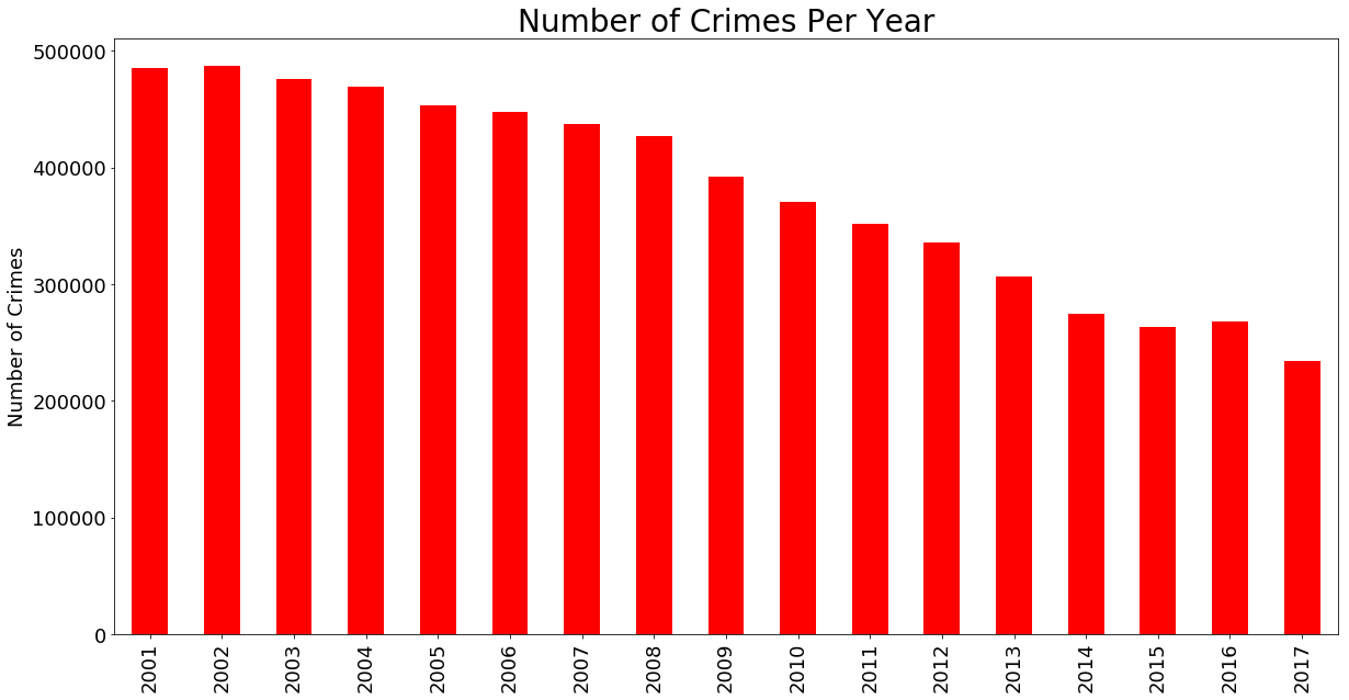
Find the number of crimes per year
df.groupBy("Year").count().show()
df.groupBy("Year").count().collect()
We can also use matplotlib and Pandas to visualize the total number of crimes per year.
count = [item[1] for item in df.groupBy("Year").count().collect()]
year = [item[0] for item in df.groupBy("Year").count().collect()]
number_of_crimes_per_year = {"count":count, "year" : year}
import pandas as pd
import matplotlib.pyplot as plt
%matplotlib inline
number_of_crimes_per_year = pd.DataFrame(number_of_crimes_per_year)
number_of_crimes_per_year.head()
count	year
0	475921	2003
1	436966	2007
2	263495	2015
3	448066	2006
4	306847	2013
number_of_crimes_per_year = number_of_crimes_per_year.sort_values(by = "year")
number_of_crimes_per_year.plot(figsize = (20,10), kind = "bar", color = "red",
                               x = "year", y = "count", legend = False)
plt.xlabel("", fontsize = 18)
plt.ylabel("Number of Crimes", fontsize = 18)
plt.title("Number of Crimes Per Year", fontsize = 28)
plt.xticks(size = 18)
plt.yticks(size = 18)
plt.show()
Gives this plot:
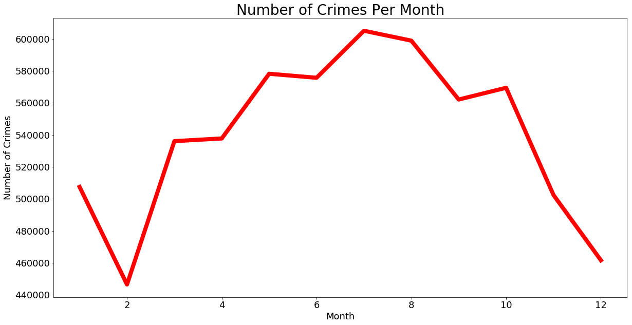
Plot number of crimes by month
from pyspark.sql.functions import month
monthdf = df.withColumn("Month",month("Date_time"))
monthCounts = monthdf.select("Month").groupBy("Month").count()
monthCounts = monthCounts.collect()
months = [item[0] for item in monthCounts]
count = [item[1] for item in monthCounts]
crimes_per_month = {"month":months, "crime_count": count}
crimes_per_month = pd.DataFrame(crimes_per_month)
crimes_per_month = crimes_per_month.sort_values(by = "month")
crimes_per_month.plot(figsize = (20,10), kind = "line", x = "month", y = "crime_count",
                      color = "red", linewidth = 8, legend = False)
plt.xlabel("Month", fontsize = 18)
plt.ylabel("Number of Crimes", fontsize = 18)
plt.title("Number of Crimes Per Month", fontsize = 28)
plt.xticks(size = 18)
plt.yticks(size = 18)
plt.show()
Gives this plot:
Where do most crimes take pace?
crime_location  = crimes.groupBy("LocationDescription").count().collect()
location = [item[0] for item in crime_location]
count = [item[1] for item in crime_location]
crime_location = {"location" : location, "count": count}
crime_location = pd.DataFrame(crime_location)
crime_location = crime_location.sort_values(by = "count", ascending  = False)
crime_location = crime_location.iloc[:20]
myplot = crime_location .plot(figsize = (20,20), kind = "barh", color = "#b35900", width = 0.8,
                               x = "location", y = "count", legend = False)
myplot.invert_yaxis()
plt.xlabel("Number of crimes", fontsize = 28)
plt.ylabel("Crime Location", fontsize = 28)
plt.title("Number of Crimes By Location", fontsize = 36)
plt.xticks(size = 24)
plt.yticks(size = 24)
plt.show()
Gives this plot:

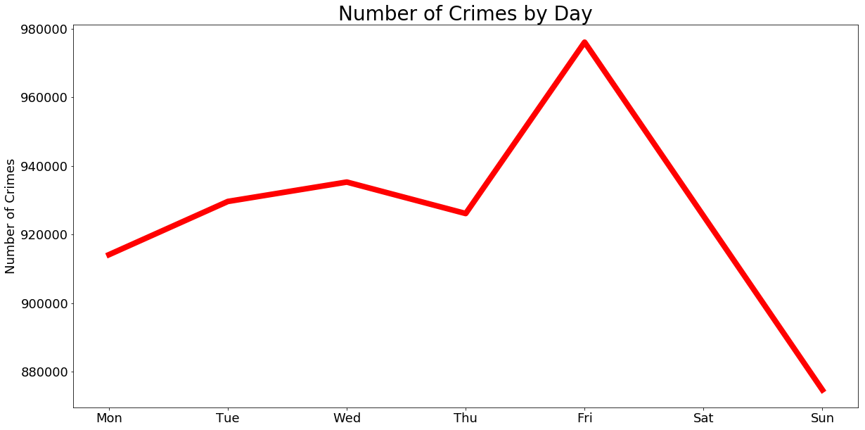
Which days have the highest number of crimes?
weekDaysCount  = df.groupBy(["DayOfWeek", "DayOfWeek_number"]).count().collect()
days = [item[0] for item in weekDaysCount]
count = [item[2] for item in weekDaysCount]
day_number = [item[1] for item in weekDaysCount]
crime_byDay = {"days" : days, "count": count, "day_number": day_number}
crime_byDay = pd.DataFrame(crime_byDay)
crime_byDay = crime_byDay.sort_values(by = "day_number", ascending  = True)


crime_byDay.plot(figsize = (20,10), kind = "line", x = "days", y = "count",
                      color = "red", linewidth = 8, legend = False)

plt.ylabel("Number of Crimes", fontsize = 18)
plt.xlabel("")
plt.title("Number of Crimes by Day", fontsize = 28)
plt.xticks(size = 18)
plt.yticks(size = 18)
plt.show()
Gives this plot:
We can also show the only number of domestic crimes by day
weekDaysCount  = df.filter(df["Domestic"] == "true").groupBy(["DayOfWeek", "DayOfWeek_number"]).count().collect()
days = [item[0] for item in weekDaysCount]
count = [item[2] for item in weekDaysCount]
day_number = [item[1] for item in weekDaysCount]
crime_byDay = {"days" : days, "count": count, "day_number": day_number}
crime_byDay = pd.DataFrame(crime_byDay)
crime_byDay = crime_byDay.sort_values(by = "days", ascending  = True)


crime_byDay.plot(figsize = (20,10), kind = "line", x = "days", y = "count",
                      color = "red", linewidth = 8, legend = False)

plt.ylabel("Number of Domestic Crimes", fontsize = 18)
plt.xlabel("")
plt.title("Number of domestic crimes by day", fontsize = 28)
plt.xticks(size = 18)
plt.yticks(size = 18)
plt.show()
Gives this plot:

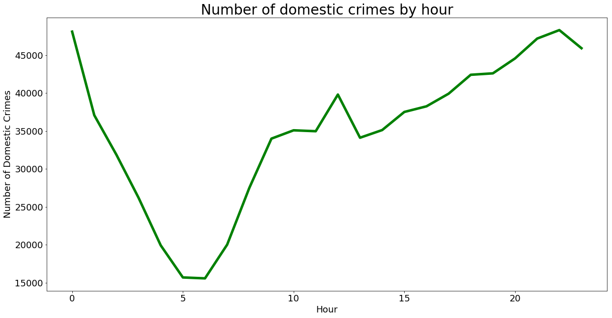
Number of domestic crimes by hour
temp = df.filter(df["Domestic"] == "true")
temp = temp.select(df['HourOfDay'].cast('int').alias('HourOfDay'))
hourlyCount  = temp.groupBy(["HourOfDay"]).count().collect()

hours = [item[0] for item in hourlyCount]
count = [item[1] for item in hourlyCount]

crime_byHour = {"count": count, "hours": hours}
crime_byHour = pd.DataFrame(crime_byHour)
crime_byHour = crime_byHour.sort_values(by = "hours", ascending  = True)


crime_byHour.plot(figsize = (20,10), kind = "line", x = "hours", y = "count",
                      color = "green", linewidth = 5, legend = False)

plt.ylabel("Number of Domestic Crimes", fontsize = 18)
plt.xlabel("Hour", fontsize = 18)
plt.title("Number of domestic crimes by hour", fontsize = 28)
plt.xticks(size = 18)
plt.yticks(size = 18)
plt.show()
Gives this plot:
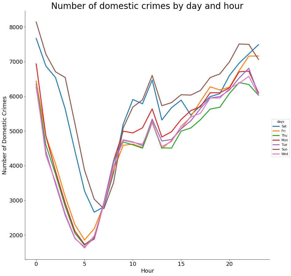
We can also show number of domestic crimes by day and hour
import seaborn as sns
temp = df.filter(df["Domestic"] == "true")
temp = temp.select("DayOfWeek", df['HourOfDay'].cast('int').alias('HourOfDay'))
hourlyCount  = temp.groupBy(["DayOfWeek","HourOfDay"]).count().collect()

days = [item[0] for item in hourlyCount]
hours = [item[1] for item in hourlyCount]
count = [item[2] for item in hourlyCount]
crime_byHour = {"count": count, "hours": hours, "days": days}
crime_byHour = pd.DataFrame(crime_byHour)
crime_byHour = crime_byHour.sort_values(by = "hours", ascending  = True)
import seaborn as sns
g = sns.FacetGrid(crime_byHour, hue="days", size = 12)
g.map(plt.plot, "hours", "count", linewidth = 3)
g.add_legend()
plt.ylabel("Number of Domestic Crimes", fontsize = 18)
plt.xlabel("Hour", fontsize = 18)
plt.title("Number of domestic crimes by day and hour", fontsize = 28)
plt.xticks(size = 18)
plt.yticks(size = 18)
plt.show()
Gives this plot:
Remarks
This is the second blog post on the Spark tutorial series to help big data enthusiasts prepare for Apache Spark Certifications from companies such as Cloudera, Hortonworks, Databricks, etc. The first one is here. If you want to learn/master Spark with Python or if you are preparing for a Spark Certification to show your skills in big data, these articles are for you.