Extreme Gradient Boosting is amongst the excited R and Python libraries in machine learning these times. Previously, I have written a tutorial on how to use Extreme Gradient Boosting with R. In this post, I will elaborate on how to conduct an analysis in Python. Extreme Gradient Boosting supports various objective functions, including regression, classification, and ranking. It has gained much popularity and attention recently as it was the algorithm of choice for many winning teams of many machine learning competitions.
This post is a continuation of my previous Machine learning with R blog post series. The first one is available here.
Import Python libraries
import xgboost as xgb
import pandas as pd
import numpy as np
import statsmodels.api as sm
from sklearn.model_selection import train_test_split
from sklearn.model_selection import GridSearchCV
from sklearn.metrics import mean_squared_error
import matplotlib.pyplot as plt
Read the data into a Pandas dataframe
power_plant = pd.read_excel("Folds5x2_pp.xlsx")
Create training and test datasets
X = power_plant.drop("PE", axis = 1)
y = power_plant['PE'].values
y = y.reshape(-1, 1)
X_train, X_test, y_train, y_test = train_test_split(X, y,test_size = 0.2, random_state=42)
Convert the training and testing sets into DMatrixes
DMatrix is the recommended class in xgboost.
DM_train = xgb.DMatrix(data = X_train,
                       label = y_train)
DM_test =  xgb.DMatrix(data = X_test,
                       label = y_test)
There are different hyperparameters that we can tune and the parametres are different from baselearner to baselearner. In tree based learners, which are the most common ones in xgboost applications, the following are the most commonly tuned hyperparameters:
learning rate:
- learning rate/eta- governs how quickly the model fits the residual error using additional base learners. If it is a smaller learning rate, it will need more boosting rounds, hence more time, to achieve the same reduction in residual error as one with larger learning rate. Typically, it lies between 0.01 – 0.3
The three hyperparameters below are regularization hyperparameters. - gamma: min loss reduction to create new tree split. default = 0 means no regularization.
- lambda: L2 reg on leaf weights. Equivalent to Ridge regression.
- alpha: L1 reg on leaf weights. Equivalent to Lasso regression.
- max_depth: max depth per tree. This controls how deep our tree can grow. The Larger the depth, more complex the model will be and higher chances of overfitting. Larger data sets require deep trees to learn the rules from data. Default = 6.
- subsample: % samples used per tree. This is the fraction of the total training set that can be used in any boosting round. Low value may lead to underfitting issues. A very high value can cause over-fitting problems.
- colsample_bytree: % features used per tree. This is the fraction of the number of columns that we can use in any boosting round. A smaller value is an additional regularization and a larger value may be cause overfitting issues.
- n_estimators: number of estimators (base learners). This is the number of boosting rounds.
In both R and Python, the default base learners are trees (gbtree) but we can also specify gblinear for linear models and dart for both classification and regression problems.
In this post, I will optimize only three of the parameters shown above and you can try optimizing the other parameters. You can see the list of parameters and their details from the website.
Parameters for grid search
gbm_param_grid = {
     'colsample_bytree': np.linspace(0.5, 0.9, 5),
     'n_estimators':[100, 200],
     'max_depth': [10, 15, 20, 25]
}
Instantiate the regressor
gbm = xgb.XGBRegressor()
Perform grid search
Let’s perform 5 fold cross-validation using mean square error as a scoring method.
grid_mse = GridSearchCV(estimator = gbm, param_grid = gbm_param_grid, scoring = 'neg_mean_squared_error', cv = 5, verbose = 1)
Fit grid_mse to the data, get best parameters and best score (lowest RMSE)
grid_mse.fit(X_train, y_train)
print("Best parameters found: ",grid_mse.best_params_)
print("Lowest RMSE found: ", np.sqrt(np.abs(grid_mse.best_score_)))
Fitting 5 folds for each of 40 candidates, totalling 200 fits
[Parallel(n_jobs=1)]: Done 200 out of 200 | elapsed: 11.0min finished
Best parameters found:  {'colsample_bytree': 0.80000000000000004, 'max_depth': 15, 'n_estimators': 200}
Lowest RMSE found:  3.03977094354
Predict using the test data
pred = grid_mse.predict(X_test)
print("Root mean square error for test dataset: {}".format(np.round(np.sqrt(mean_squared_error(y_test, pred)), 2)))
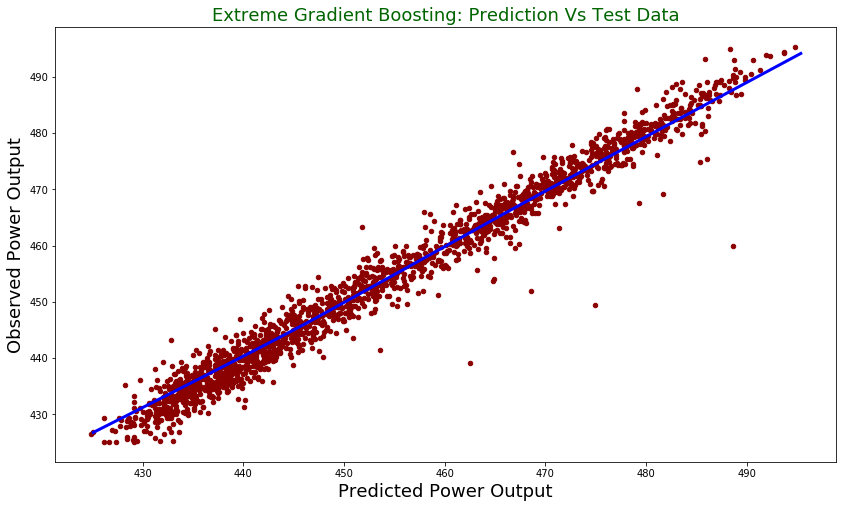
Root mean square error for test dataset: 2.76
test = pd.DataFrame({"prediction": pred, "observed": y_test.flatten()})
lowess = sm.nonparametric.lowess
z = lowess(pred.flatten(), y_test.flatten())
test.plot(figsize = [14,8],
          x ="prediction", y = "observed", kind = "scatter", color = 'darkred')
plt.title("Extreme Gradient Boosting: Prediction Vs Test Data", fontsize = 18, color = "darkgreen")
plt.xlabel("Predicted Power Output", fontsize = 18)
plt.ylabel("Observed Power Output", fontsize = 18)
plt.plot(z[:,0], z[:,1], color = "blue", lw= 3)
plt.show()
The plot:
Summary
In this post, I used python to run Extreme Gradient Boosting to predict power output. We see that it has better performance than linear model we tried in the first part of the blog post series.
Why did you reshape the y as (-1,1). I didn’t understand that step. Please message me at [email protected]
what’s the point of Dmatrix? I don’t see you use these two datasets afterwards?
where is the data “Folds5x2_pp.xlsx”?