Extreme Gradient Boosting is among the hottest libraries in supervised machine learning these days. It supports various objective functions, including regression, classification, and ranking. It has gained much popularity and attention recently as it was the algorithm of choice for many winning teams of a number of machine learning competitions.
What makes it so popular are its speed and performance. It gives among the best performances in many machine learning applications. It is optimized gradient-boosting machine learning library. The core algorithm is parallelizable and hence it can use all the processing power of your machine and the machines in your cluster. In R, according to the package documentation, since the package can automatically do parallel computation on a single machine, it could be more than 10 times faster than existing gradient boosting packages.
xgboost shines when we have lots of training data where the features are numeric or a mixture of numeric and categorical fields. It is also important to note that xgboost is not the best algorithm out there when all the features are categorical or when the number of rows is less than the number of fields (columns).
For other applications such as image recognition, computer vision or natural language processing, xgboost is not the ideal library. Do not use xgboost for small size dataset. It has libraries in Python, R, Julia, etc. In this post, we will see how to use it in R.
This post is a continuation of my previous Machine learning with R blog post series. The first one is available here. Data exploration was performed in the first part, so I will not repeat it here.
We will use the caret package for cross-validation and grid search.
Load packages
library(readxl)
library(tidyverse)
library(xgboost)
library(caret)
Read Data
power_plant = as.data.frame(read_excel("Folds5x2_pp.xlsx"))
Create training set indices with 80% of data: we are using the caret package to do this
set.seed(100)  # For reproducibility
# Create index for testing and training data
inTrain <- createDataPartition(y = power_plant$PE, p = 0.8, list = FALSE)
# subset power_plant data to training
training <- power_plant[inTrain,]
# subset the rest to test
 testing <- power_plant[-inTrain,]
Convert the training and testing sets into DMatrixes: DMatrix is the recommended class in xgboost.
X_train = xgb.DMatrix(as.matrix(training %>% select(-PE)))
y_train = training$PE
X_test = xgb.DMatrix(as.matrix(testing %>% select(-PE)))
y_test = testing$PE
Specify cross-validation method and number of folds. Also enable parallel computation
xgb_trcontrol = trainControl(
  method = "cv",
  number = 5,
  allowParallel = TRUE,
  verboseIter = FALSE,
  returnData = FALSE
)
This is the grid space to search for the best hyperparameters
I am specifing the same parameters with the same values as I did for Python above. The hyperparameters to optimize are found in the website.
xgbGrid <- expand.grid(nrounds = c(100,200),  # this is n_estimators in the python code above
                       max_depth = c(10, 15, 20, 25),
                       colsample_bytree = seq(0.5, 0.9, length.out = 5),
                       ## The values below are default values in the sklearn-api.
                       eta = 0.1,
                       gamma=0,
                       min_child_weight = 1,
                       subsample = 1
                      )
Finally, train your model
set.seed(0)
xgb_model = train(
  X_train, y_train,
  trControl = xgb_trcontrol,
  tuneGrid = xgbGrid,
  method = "xgbTree"
)
Best values for hyperparameters
xgb_train$bestTune
nrounds	max_depth	eta	gamma	colsample_bytree	min_child_weight	subsample
18	200	15	0.1	0	0.8	1	1
We see above that we get the same hyperparameter values from both R and Python.
Model evaluation
predicted = predict(xgb_model, X_test)
residuals = y_test - predicted
RMSE = sqrt(mean(residuals^2))
cat('The root mean square error of the test data is ', round(RMSE,3),'\n')
The root mean square error of the test data is 2.856
y_test_mean = mean(y_test)
# Calculate total sum of squares
tss =  sum((y_test - y_test_mean)^2 )
# Calculate residual sum of squares
rss =  sum(residuals^2)
# Calculate R-squared
rsq  =  1 - (rss/tss)
cat('The R-square of the test data is ', round(rsq,3), '\n')
The R-square of the test data is 0.972
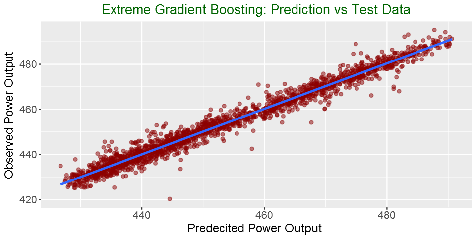
Plotting actual vs predicted
options(repr.plot.width=8, repr.plot.height=4)
my_data = as.data.frame(cbind(predicted = predicted,
                            observed = y_test))
# Plot predictions vs test data
ggplot(my_data,aes(predicted, observed)) + geom_point(color = "darkred", alpha = 0.5) +
    geom_smooth(method=lm)+ ggtitle('Linear Regression ') + ggtitle("Extreme Gradient Boosting: Prediction vs Test Data") +
      xlab("Predecited Power Output ") + ylab("Observed Power Output") +
        theme(plot.title = element_text(color="darkgreen",size=16,hjust = 0.5),
         axis.text.y = element_text(size=12), axis.text.x = element_text(size=12,hjust=.5),
         axis.title.x = element_text(size=14), axis.title.y = element_text(size=14))
Summary
In this post, We used Extreme Gradient Boosting to predict power output. We see that it has better performance than linear model we tried in the first part of the blog post series. The RMSE with the test data decreased from more 4.4 to 2.8. See you in the next part of my machine learning blog post.
Could you share the excel?
Thanks for good posting!
I have one question of my problem.
When I tried to execute the code below, error message occurred.
xgb_model = train(
dtrain, dtest,
trControl = xgb_trcontrol,
tuneGrid = xgbGrid,
method = “xgbTree”
)
Error in train(dtrain, dtest, trControl = xgb_trcontrol, tuneGrid = xgbGrid, :
unused arguments (trControl = xgb_trcontrol, tuneGrid = xgbGrid, method = “xgbTree”)
How can I deal with error?
Could you help me?
Excellent post!, thanks
xgb_train$bestTune
should probably be
xgb_model$bestTune
it is correct
Hi,
what does the model provide? probabilities?
Always nice to read your blog