We know that Amazon Product Reviews Matter to Merchants because those reviews have a tremendous impact on how we make purchase decisions. So, I downloaded an Amazon fine food reviews data set from Kaggle that originally came from SNAP, to see what I could learn from this large data set.
Our aim here isn’t to achieve Scikit-Learn mastery, but to explore some of the main Scikit-Learn tools on a single CSV file: by analyzing a collection of text documents (568,454 food reviews) up to and including October 2012. Let’s get started.
Data
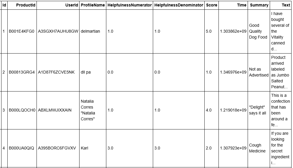
Looking at the head of the data frame, we can see that it consists of the following information:
-
1. Product Id
2. User Id
3. ProfileName
4. HelpfulnessNumerator
5. HelpfulnessDenominator
6. Score
7. Time
8. Summary
9. Text
import pandas as pd
import numpy as np

df = pd.read_csv('Reviews.csv')
df.head()
For our purpose today, we will be focusing on Score and Text columns.
Let’s start by cleaning up the data frame, by dropping any rows that have missing values.
The Score column is scaled from 1 to 5, and we will remove all Scores equal to 3 because we assume these are neutral and did not provide us any useful information. We then add a new column called “Positivity”, where any score above 3 is encoded as a 1, indicating it was positively rated. Otherwise, it’ll be encoded as a 0, indicating it was negatively rated.
df.dropna(inplace=True)
df[df['Score'] != 3]
df['Positivity'] = np.where(df['Score'] > 3, 1, 0)
df.head()
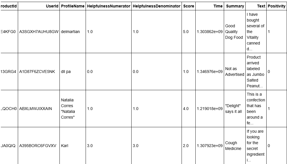
It looks good.
Now, let’s split our data into random training and test subsets using “Text” and “Positivity” columns, and then print out the first entry and the shape of the training set.
from sklearn.model_selection import train_test_split
X_train, X_test, y_train, y_test = train_test_split(df['Text'], df['Positivity'], random_state = 0)
print('X_train first entry: \n\n', X_train[0])
print('\n\nX_train shape: ', X_train.shape)
from sklearn.model_selection import train_test_split
X_train, X_test, y_train, y_test = train_test_split(df['Text'], df['Positivity'], random_state = 0)
print('X_train first entry: \n\n', X_train[0])
print('\n\nX_train shape: ', X_train.shape)
X_train first entry:
I have bought several of of the Vitality canned dog food products and have found them all to be of good quality. The product looks more like a stew than a processed meat and it smells better. My Labrador is finicky and she appreciates this product better than most.
X_train shape: (26377,)
Looking at X_train, we can see that we have a collection of over 26000 reviews or documents. In order to perform machine learning on text documents, we first need to turn these text content into numerical feature vectors that Scikit-Learn can use.
Bags-of-words
The simplest and most intuitive way to do so is the “bags-of-words” representation which ignores structure and simply counts how often each word occurs. CountVectorizer allows us to use the bags-of-words approach, by converting a collection of text documents into a matrix of token counts.
We instantiate the CountVectorizer and fit it to our training data, converting our collection of text documents into a matrix of token counts.
from sklearn.feature_extraction.text import CountVectorizer
vect = CountVectorizer().fit(X_train)
vect
CountVectorizer(analyzer=’word’, binary=False, decode_error=’strict’,dtype=, encoding=’utf-8',input=’content’,lowercase=True, max_df=1.0, max_features=None, min_df=1,ngram_range=(1, 1), preprocessor=None, stop_words=None,strip_accents=None, token_pattern=’(?u)\\b\\w\\w+\\b’,tokenizer=None, vocabulary=None)
This model has many parameters, however, the default values are quite reasonable for our purpose.
The default configuration tokenizes the string, by extracting words of at least 2 letters or numbers, separated by word boundaries, it then converts everything to lowercase and builds a vocabulary using these tokens. We can get some of the vocabularies by using the get_feature_names method like so:
vect.get_feature_names()[::2000]
[‘00’, ‘anyonr’, ‘bleaching’, ‘chunky’, ‘defeated’, ‘er’, ‘giannini’, ‘impresses’, ‘little’, ‘necklace’, ‘pets’, ‘reduced’, ‘shirts’, ‘supper’, ‘unedible’]
Looking at those vocabularies, we can get a small sense of what they are about. By checking the length of get_feature_names, we can see that we’re working with 29990 features.
len(vect.get_feature_names())
29990
Next, we transform the documents in X_train to a document term matrix, which gives us the bags-of-word representation of X_train. The result is stored in a SciPy sparse matrix, where each row corresponds to a document, and each column is a word from our training vocabulary.
X_train_vectorized = vect.transform(X_train)
X_train_vectorized
<26377x29990 sparse matrix of type ‘’with 1406227 stored elements in Compressed Sparse Row format>
This interpretation of the columns can be retrieved as follows:
X_train_vectorized.toarray()
array([[0, 0, 0, ..., 0, 0, 0],
       [0, 0, 0, ..., 0, 0, 0],
       [0, 0, 0, ..., 0, 0, 0],
       ...,
       [0, 0, 0, ..., 0, 0, 0],
       [0, 0, 0, ..., 0, 0, 0],
       [0, 0, 0, ..., 0, 0, 0]], dtype=int64)
The entries in this matrix are the number of times each word appears in each document. Because the number of words in the vocabulary is so much larger than the number of words that might appear in a single text, most entries of this matrix are zero.
Logistic Regression
Now, we will train the Logistic Regression classifier based on this feature matrix X_ train_ vectorized because Logistics Regression works well for high dimensional sparse data.
from sklearn.linear_model import LogisticRegression
model = LogisticRegression()
model.fit(X_train_vectorized, y_train)
LogisticRegression(C=1.0, class_weight=None, dual=False, fit_intercept=True, intercept_scaling=1, max_iter=100, multi_class=’ovr’, n_jobs=1, penalty=’l2', random_state=None, solver=’liblinear’, tol=0.0001, verbose=0, warm_start=False)
Next, we’ll make predictions using X_test, and compute the area under the curve score.
from sklearn.metrics import roc_auc_score
predictions = model.predict(vect.transform(X_test))
print('AUC: ', roc_auc_score(y_test, predictions))
AUC: 0.797745838184
The result is not bad. In order to better understand how our model makes these predictions, we can use the coefficients for each feature (a word) to determine its weight in terms of positivity and negativity.
feature_names = np.array(vect.get_feature_names())
sorted_coef_index = model.coef_[0].argsort()
print('Smallest Coefs: \n{}\n'.format(feature_names[sorted_coef_index[:10]]))
print('Largest Coefs: \n{}\n'.format(feature_names[sorted_coef_index[:-11:-1]]))
Smallest Coefs: [‘worst’ ‘disappointing’ ‘horrible’ ‘awful’ ‘ok’ ‘neither’ ‘shame’ ‘unfortunately’ ‘disappointment’ ‘disgusting’]
Largest Coefs: [‘hooked’ ‘bright’ ‘delicious’ ‘amazing’ ‘skeptical’ ‘worried’ ‘yum’ ‘excellent’ ‘reorder’ ‘yummy’]
Sorting the ten smallest and ten largest coefficients, we can see the model has predicted words like “worst”, “disappointing” and “horrible” to negative reviews, and words like “hooked”, “bright”, and “delicious” to positive reviews.
However, our model can be improved.
Tf–idf term weighting
In a large text corpus, some words will be present very often but will carry very little meaningful information about the actual contents of the document (such as “the”, “a” and “is”). If we were to feed the count data directly to a classifier those very frequent terms would shadow the frequencies of rarer yet more interesting terms. Tf-idf allows us to weight terms based on how important they are to a document.
So, we will instantiate the tf–idf vectorizer and fit it to our training data. We specify min_df = 5, which will remove any words from our vocabulary that appear in fewer than five documents.
from sklearn.feature_extraction.text import TfidfVectorizer
vect = TfidfVectorizer(min_df = 5).fit(X_train)
len(vect.get_feature_names())
9680
X_train_vectorized = vect.transform(X_train)
model = LogisticRegression()
model.fit(X_train_vectorized, y_train)
predictions = model.predict(vect.transform(X_test))
print('AUC: ', roc_auc_score(y_test, predictions))
AUC: 0.759768072872
So, although we were able to reduce the number of features from 29990 to just 9680, our AUC score dropped by almost 4%.
Using the following code, we are able to obtain a list of features with the smallest tf-idf that either commonly appeared across all reviews or only appeared rarely in very long reviews and a list of features with the largest tf–idf contains words which appeared frequently in a review, but did not appear commonly across all reviews.
feature_names = np.array(vect.get_feature_names())
sorted_tfidf_index = X_train_vectorized.max(0).toarray()[0].argsort()
print('Smallest Tfidf: \n{}\n'.format(feature_names[sorted_tfidf_index[:10]]))
print('Largest Tfidf: \n{}\n'.format(feature_names[sorted_tfidf_index[:-11:-1]]))
Smallest Tfidf: [‘blazin’ ‘4thd’ ‘nations’ ‘committee’ ‘300mgs’ ‘350mgs’ ‘sciences’ ‘biochemical’ ‘nas’ ‘fnb’]
Largest Tfidf: [‘mustard’ ‘br’ ‘jerk’ ‘tang’ ‘chili’ ‘wound’ ‘caviar’ ‘salsa’ ‘litter’ ‘el’]
Let’s test our model:
print(model.predict(vect.transform(['The candy is not good, I will never buy them again','The candy is not bad, I will buy them again'])))
[1 0]
Our current model misclassified the document “The candy is not good, I will never buy them again” as a positive review, and it also misclassified the document “The candy is not bad, I will buy them again” as a negative review.
n-grams
One way to fix this misclassification is to add n-grams. For example, bigrams count pairs of adjacent words and could give us features such as bad versus not bad. Thus, we are refitting our training set specifying a minimum document frequency of 5 and extracting 1-grams and 2-grams.
vect = CountVectorizer(min_df = 5, ngram_range = (1,2)).fit(X_train)
X_train_vectorized = vect.transform(X_train)
len(vect.get_feature_names())
61958
Now we get a lot more features to work with but our AUC score increased:
model = LogisticRegression()
model.fit(X_train_vectorized, y_train)
predictions = model.predict(vect.transform(X_test))
print('AUC: ', roc_auc_score(y_test, predictions))
AUC: 0.838772959029
Using the coefficients to check each feature, we can see
feature_names = np.array(vect.get_feature_names())
sorted_coef_index = model.coef_[0].argsort()
print('Smallest Coef: \n{}\n'.format(feature_names[sorted_coef_index][:10]))
print('Largest Coef: \n{}\n'.format(feature_names[sorted_coef_index][:-11:-1]))
Smallest Coef: [‘worst’ ‘ok’ ‘not recommend’ ‘not worth’ ‘awful’ ‘at best’ ‘unfortunately’ ‘terrible’ ‘very disappointed’ ‘disappointing’]
Largest Coef: [‘delicious’ ‘amazing’ ‘not too’ ‘excellent’ ‘be disappointed’ ‘not bitter’ ‘yummy’ ‘hooked’ ‘great’ ‘love this’]
Our new model has correctly predicted bigrams like “not recommend”, “not worth” to negative reviews, and bigrams like “not bitter”, “not too” to positive reviews.
Let’s test our new model:
print(model.predict(vect.transform(['The candy is not good, I would never buy them again','The candy is not bad, I will buy them again'])))
[0 1]
Our latest model now correctly identifies them as negative and positive reviews respectively.
Try yourself
I hope you enjoyed this article, and have fun practicing machine learning skills on text data! Feel free to leave feedback or questions.
Reference: Scikit-Learn