Performing SQL selects on R data frames

For anyone who has SQL background and who wants to learn R, I guess the sqldf package is very useful because it enables us to use SQL commands in R. One who has basic SQL skills can manipulate data frames in R using their SQL skills. You can read more about sqldf package from cran.

In this post, we will see how to perform joins and other queries to retrieve, sort and filter data in R using SQL. We will also see how we can achieve the same tasks using non-SQL R commands. Currently, I am working with the FDA adverse events data. These data sets are ideal for a data scientist or for any data enthusiast to work with because they contain almost any kind of data messiness: missing values, duplicates, compatibility problems of data sets created during different time periods, variable names and number of variables changing over time (e.g., sex in one dataset, gender in other dataset, if_cod in one dataset and if_code in other dataset), missing errors, etc.

In this post, we will use FDA adverse events data, which are publicly available.The FDA adverse events datasets can also be downloaded in .csv format from the National Bureau of Economic Research. Since, it is easier to automate the data download in R from the National Bureau of Economic Research, we will download various datasets from this website. I encourage you to try the R codes and download data from the website and explore the adverse events datasets.

The adverse events datasets are created in quarterly temporal resolution and each quarter data includes demography information, drug/biologic information, adverse event, outcome and diagnosis, etc.

Let’s download some datasets and use SQL queries to join, sort and filter the various data frames.

Load R Packages

require(downloader)
library(dplyr)
library(sqldf)
library(data.table)
library(ggplot2)
library(compare)
library(plotrix)

Basic error Handing with tryCatch()

We will use the function below to download data. Since the data sets have quarterly time resolution, there are four data sets per year for each observation. So, the function below will automate the data dowlnoad. If the quartely data is not available on the website (not yet released), the function will give an error message that the dataset was not found. We are downloading zipped data and unzipping it.

try.error = function(url)
{
  try_error = tryCatch(download(url,dest="data.zip"), error=function(e) e)
  if (!inherits(try_error, "error")){
      download(url,dest="data.zip")
        unzip ("data.zip")
      }
    else if (inherits(try_error, "error")){
    cat(url,"not found\n")
      }
      }

Download adverse events data

The FDA adverse events data are available since 2004. In this post, let’s download data since 2013. We will check if there are data up to the present time and download what we can get.

Sys.time() gives the current date and time
the function year() from the data.table package gets the year from the current date and time data that we obtain from the Sys.time() function

We are downloading demography, drug, diagnosis/indication, outcome and reaction (adeverse event) data.

year_start=2013
year_last=year(Sys.time())
for (i in year_start:year_last){
            j=c(1:4)
            for (m in j){
            url1<-paste0("http://www.nber.org/fda/faers/",i,"/demo",i,"q",m,".csv.zip")
            url2<-paste0("http://www.nber.org/fda/faers/",i,"/drug",i,"q",m,".csv.zip")
            url3<-paste0("http://www.nber.org/fda/faers/",i,"/reac",i,"q",m,".csv.zip")
            url4<-paste0("http://www.nber.org/fda/faers/",i,"/outc",i,"q",m,".csv.zip")
            url5<-paste0("http://www.nber.org/fda/faers/",i,"/indi",i,"q",m,".csv.zip")
           try.error(url1)
           try.error(url2)
           try.error(url3)
           try.error(url4)
           try.error(url5)     
            }
        }
http://www.nber.org/fda/faers/2015/demo2015q4.csv.zip not found
...
http://www.nber.org/fda/faers/2016/indi2016q4.csv.zip not found

From the error messages shown above, in the time of writing this post, we see that the database has adverse events data up to the third quarter of 2015.

list.files() produce a character vector of the names of files in my working directory.
I am using regular expressions to select each categoy of dateset. Example, ^demo.*.csv means all files that start with the word demo and end with .csv.

filenames <- list.files(pattern="^demo.*.csv", full.names=TRUE)
cat('We have downloaded the following quarterly demography datasets')
filenames

We have downloaded the following quarterly demography datasets

"./demo2012q1.csv" "./demo2012q2.csv" "./demo2012q3.csv" "./demo2012q4.csv" "./demo2013q1.csv" "./demo2013q2.csv" "./demo2013q3.csv" "./demo2013q4.csv" "./demo2014q1.csv" "./demo2014q2.csv" "./demo2014q3.csv" "./demo2014q4.csv" "./demo2015q1.csv" "./demo2015q2.csv" "./demo2015q3.csv"

Now let’s use fread() function from the data.table Package to read in the datasets. Let’s start with the demography data:

demo=lapply(filenames,fread)

Now, let’s change them to data frames and concatenate them to create one demography data

demo_all=do.call(rbind,lapply(1:length(demo),function(i) select(as.data.frame(demo[i]),primaryid,caseid, age,age_cod,event_dt,sex,reporter_country)))
dim(demo_all)
3554979   7

We see that our demography data has more than 3.5 million rows.

Now, lets’ merge all drug files

filenames <- list.files(pattern="^drug.*.csv", full.names=TRUE)
cat('We have downloaded the following quarterly drug datasets:\n')
filenames
drug=lapply(filenames,fread)
cat('\n')
cat('Variable names:\n')
names(drug[[1]])
drug_all=do.call(rbind,lapply(1:length(drug), function(i) select(as.data.frame(drug[i]),primaryid,caseid, drug_seq,drugname,route)))

We have downloaded the following quarterly drug datasets:

"./drug2012q1.csv" "./drug2012q2.csv" "./drug2012q3.csv" 
"./drug2012q4.csv" "./drug2013q1.csv" "./drug2013q2.csv" 
"./drug2013q3.csv" "./drug2013q4.csv" "./drug2014q1.csv" 
"./drug2014q2.csv" "./drug2014q3.csv" "./drug2014q4.csv" 
"./drug2015q1.csv" "./drug2015q2.csv" "./drug2015q3.csv"

Variable names:

"primaryid" "drug_seq" "role_cod" "drugname" 
"val_vbm" "route" "dose_vbm" "dechal" "rechal" "lot_num" 
"exp_dt" "exp_dt_num" "nda_num"

Merge all diagnoses/indications datasets

filenames <- list.files(pattern="^indi.*.csv", full.names=TRUE)
cat('We have downloaded the following quarterly diagnoses/indications datasets:\n')

filenames

indi=lapply(filenames,fread)

cat('\n')
cat('Variable names:\n')

names(indi[[15]])

indi_all=do.call(rbind,lapply(1:length(indi), function(i) select(as.data.frame(indi[i]),primaryid,caseid, indi_drug_seq,indi_pt)))

We have downloaded the following quarterly diagnoses/indications datasets:

"./indi2012q1.csv" "./indi2012q2.csv" "./indi2012q3.csv" "./indi2012q4.csv" "./indi2013q1.csv" "./indi2013q2.csv" "./indi2013q3.csv" "./indi2013q4.csv" "./indi2014q1.csv" "./indi2014q2.csv" "./indi2014q3.csv" "./indi2014q4.csv" "./indi2015q1.csv" "./indi2015q2.csv" "./indi2015q3.csv"

Variable names:

"primaryid" "caseid" "indi_drug_seq" "indi_pt"

Merge patient outcomes

filenames <- list.files(pattern="^outc.*.csv", full.names=TRUE)
cat('We have downloaded the following quarterly patient outcome datasets:\n')

filenames
outc_all=lapply(filenames,fread)

cat('\n')
cat('Variable names\n')

names(outc_all[[1]])
names(outc_all[[4]])
colnames(outc_all[[4]])=c("primaryid", "caseid", "outc_cod")
outc_all=do.call(rbind,lapply(1:length(outc_all), function(i) select(as.data.frame(outc_all[i]),primaryid,outc_cod)))

We have downloaded the following quarterly patient outcome datasets:

"./outc2012q1.csv" "./outc2012q2.csv" "./outc2012q3.csv" "./outc2012q4.csv" "./outc2013q1.csv" "./outc2013q2.csv" "./outc2013q3.csv" "./outc2013q4.csv" "./outc2014q1.csv" "./outc2014q2.csv" "./outc2014q3.csv" "./outc2014q4.csv" "./outc2015q1.csv" "./outc2015q2.csv" "./outc2015q3.csv"

Variable names

"primaryid" "outc_cod" 
    "primaryid" "caseid" "outc_code"

Finally, merge reaction (adverse event) datasets

filenames <- list.files(pattern="^reac.*.csv", full.names=TRUE)
cat('We have downloaded the following quarterly reaction (adverse event)  datasets:\n')

filenames
reac=lapply(filenames,fread)

cat('\n')
cat('Variable names:\n')
names(reac[[3]])

reac_all=do.call(rbind,lapply(1:length(indi), function(i) select(as.data.frame(reac[i]),primaryid,pt)))

We have downloaded the following quarterly reaction (adverse event) datasets:

"./reac2012q1.csv" "./reac2012q2.csv" "./reac2012q3.csv" "./reac2012q4.csv" "./reac2013q1.csv" "./reac2013q2.csv" "./reac2013q3.csv" "./reac2013q4.csv" "./reac2014q1.csv" "./reac2014q2.csv" "./reac2014q3.csv" "./reac2014q4.csv" "./reac2015q1.csv" "./reac2015q2.csv" "./reac2015q3.csv"

Variable names:

"primaryid" "pt"

Let’s see number of rows from each data type

all=as.data.frame(list(Demography=nrow(demo_all),Drug=nrow(drug_all),
                   Indications=nrow(indi_all),Outcomes=nrow(outc_all),
                   Reactions=nrow(reac_all)))
row.names(all)='Number of rows'
all

SQL queries

Keep in mind that sqldf uses SQLite.

COUNT

#SQL
sqldf("SELECT COUNT(primaryid)as 'Number of rows of Demography data'
FROM demo_all;")

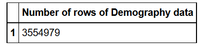
# R
nrow(demo_all)
3554979

LIMIT

#  SQL
sqldf("SELECT *
FROM demo_all 
LIMIT 6;")

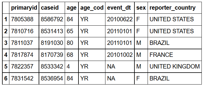
#R
head(demo_all,6)

R1=head(demo_all,6)
SQL1 =sqldf("SELECT *
FROM demo_all 
LIMIT 6;")
all.equal(R1,SQL1)
TRUE

WHERE

SQL2=sqldf("SELECT *
FROM demo_all WHERE sex ='F';")
R2 = filter(demo_all, sex=="F")
identical(SQL2, R2)
TRUE

SQL3=sqldf("SELECT *
FROM demo_all WHERE age BETWEEN 20 AND 25;")
R3 = filter(demo_all, age >= 20 & age <= 25)
identical(SQL3, R3)
TRUE

GROUP BY and ORDER BY

#SQL
sqldf("SELECT sex, COUNT(primaryid) as Total
FROM demo_all
WHERE sex IN ('F','M','NS','UNK')
GROUP BY sex
ORDER BY Total DESC ;")

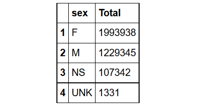
# R
demo_all%>%filter(sex %in%c('F','M','NS','UNK'))%>%group_by(sex) %>%
        summarise(Total = n())%>%arrange(desc(Total))

SQL3 = sqldf("SELECT sex, COUNT(primaryid) as Total
FROM demo_all
GROUP BY sex
ORDER BY Total DESC ;")

R3 = demo_all%>%group_by(sex) %>%
        summarise(Total = n())%>%arrange(desc(Total))

compare(SQL3,R3, allowAll=TRUE)
TRUE
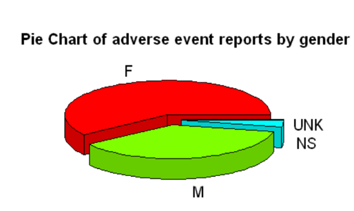
  dropped attributes

SQL=sqldf("SELECT sex, COUNT(primaryid) as Total
FROM demo_all
WHERE sex IN ('F','M','NS','UNK')
GROUP BY sex
ORDER BY Total DESC ;")
SQL$Total=as.numeric(SQL$Total
pie3D(SQL$Total, labels = SQL$sex,explode=0.1,col=rainbow(4),
   main="Pie Chart of adverse event reports by gender",cex.lab=0.5, cex.axis=0.5, cex.main=1,labelcex=1)

This is the plot:

Inner Join

Let’s join drug data and indication data based on primary id and drug sequence
First, let’s check the variable names to see how to merge the two datasets.

names(indi_all)
names(drug_all)
names(indi_all)=c("primaryid", "drug_seq", "indi_pt" ) # so as to have the same name (drug_seq)
R4= merge(drug_all,indi_all, by = intersect(names(drug_all), names(indi_all)))
R4=arrange(R3, primaryid,drug_seq,drugname,indi_pt)
SQL4= sqldf("SELECT d.primaryid as primaryid, d.drug_seq as drug_seq, d.drugname as drugname,
                       d.route as route,i.indi_pt as indi_pt
                       FROM drug_all d
                       INNER JOIN indi_all i
                      ON d.primaryid= i.primaryid AND d.drug_seq=i.drug_seq
                      ORDER BY primaryid,drug_seq,drugname, i.indi_pt")
compare(R4,SQL4,allowAll=TRUE)
R5 = merge(reac_all,outc_all,by=intersect(names(reac_all), names(outc_all)))
SQL5 =reac_outc_new4=sqldf("SELECT r.*, o.outc_cod as outc_cod
                     FROM reac_all r 
                     INNER JOIN outc_all o
                     ON r.primaryid=o.primaryid
                     ORDER BY r.primaryid,r.pt,o.outc_cod")

compare(R5,SQL5,allowAll = TRUE)
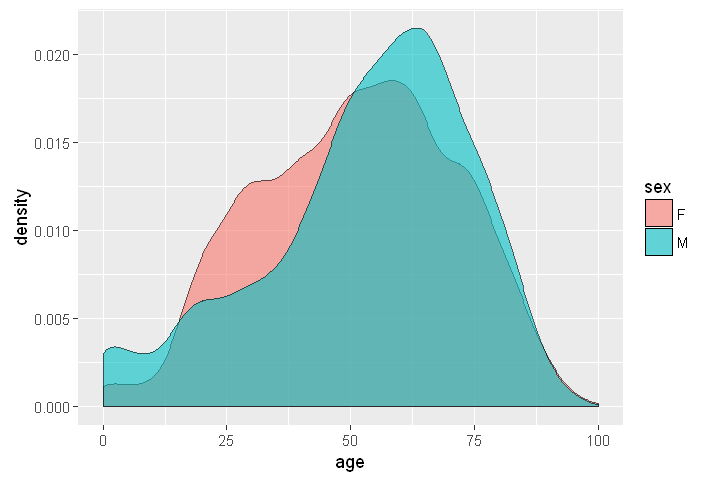
ggplot(sqldf('SELECT age, sex
             FROM demo_all
             WHERE age between 0 AND 100 AND sex IN ("F","M")
             LIMIT 10000;'), aes(x=age, fill = sex))+ geom_density(alpha = 0.6)
"primaryid" "indi_drug_seq" "indi_pt" 
    "primaryid" "drug_seq" "drugname" "route" 
TRUE
TRUE

This is the plot:

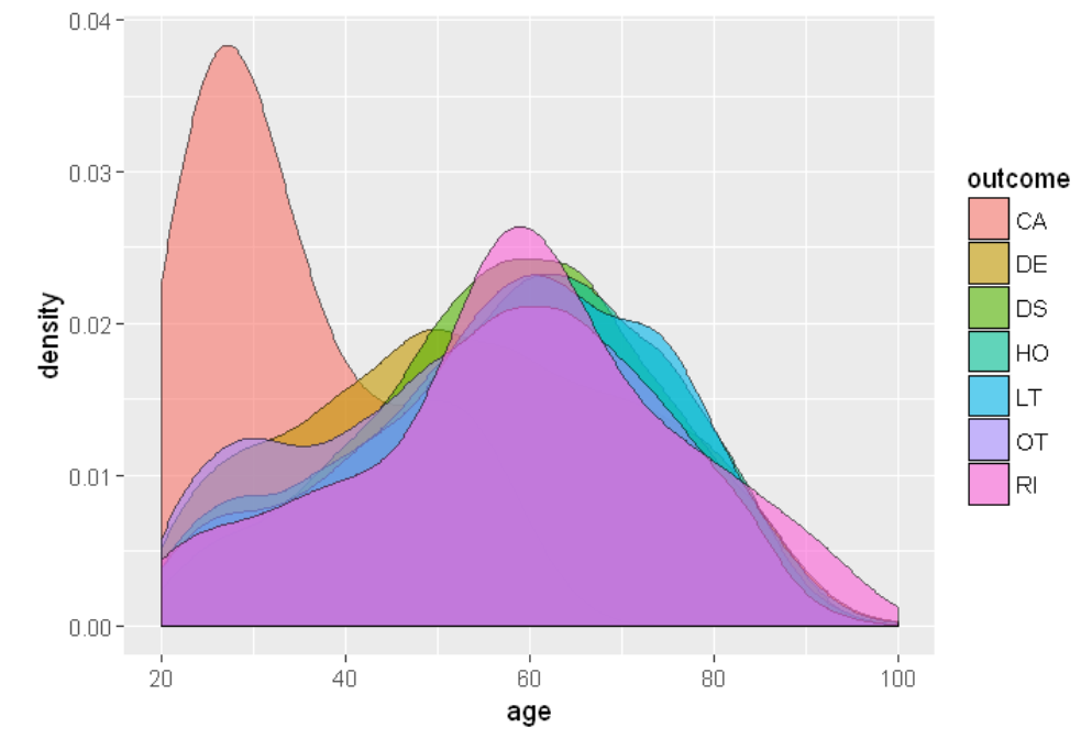
ggplot(sqldf("SELECT d.age as age, o.outc_cod as outcome
                     FROM demo_all d
                     INNER JOIN outc_all o
                     ON d.primaryid=o.primaryid
                     WHERE d.age BETWEEN 20 AND 100
                     LIMIT 20000;"),aes(x=age, fill = outcome))+ geom_density(alpha = 0.6)

This is the plot:

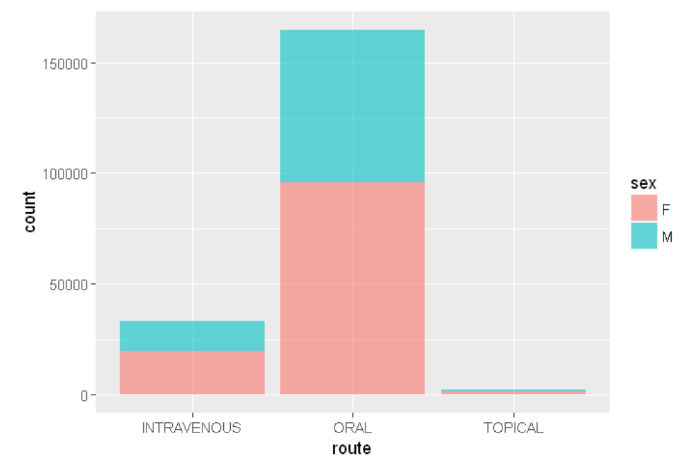
ggplot(sqldf("SELECT de.sex as sex, dr.route as route
                     FROM demo_all de
                     INNER JOIN drug_all dr
                     ON de.primaryid=dr.primaryid
                     WHERE de.sex IN ('M','F') AND dr.route IN ('ORAL','INTRAVENOUS','TOPICAL')
                     LIMIT 200000;"),aes(x=route, fill = sex))+ geom_bar(alpha=0.6)

This is the plot:

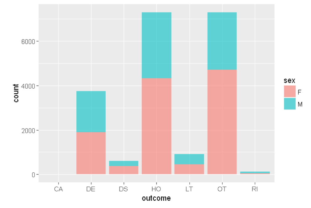
ggplot(sqldf("SELECT d.sex as sex, o.outc_cod as outcome
                     FROM demo_all d
                     INNER JOIN outc_all o
                     ON d.primaryid=o.primaryid
                     WHERE d.age BETWEEN 20 AND 100 AND sex IN ('F','M')
                     LIMIT 20000;"),aes(x=outcome,fill=sex))+ geom_bar(alpha = 0.6)

This is the plot:

demo1= demo_all[1:20000,]
demo2=demo_all[20001:40000,]

UNION ALL

R6 <- rbind(demo1, demo2)
SQL6 <- sqldf("SELECT  * FROM demo1 UNION ALL SELECT * FROM demo2;")
compare(R6,SQL6, allowAll = TRUE)
TRUE

INTERSECT

R7 <- semi_join(demo1, demo2)
SQL7 <- sqldf("SELECT  * FROM demo1 INTERSECT SELECT * FROM demo2;")
compare(R7,SQL7, allowAll = TRUE)
TRUE

EXCEPT

R8 <- anti_join(demo1, demo2)
SQL8 <- sqldf("SELECT  * FROM demo1 EXCEPT SELECT * FROM demo2;")
compare(R8,SQL8, allowAll = TRUE)
TRUE

See you in my next post! If you have any questions or feedback, feel free to leave a comment.

Data FramesData ManipulationSQL