Parsing Text for Emotion Terms: Analysis & Visualization Using R

Recently, I read a post regarding a sentiment analysis of Mr Warren Buffett’s annual shareholder letters in the past 40 years written by Michael Toth. In this post, only five of the annual shareholder letters showed negative net sentiment scores, whereas a majority of the letters (88%) displayed a positive net sentiment score. Toth noted that the years with negative net sentiment scores (1987, 1990, 2001, 2002 and 2008), coincided with lower annual returns on investments and global market decline. This observation caught my attention and triggered my curiosity about emotion words in those same shareholder letters, and whether or not emotion words were differentially expressed among the 40 letters.

With the explosion of digital and social media, there are various emoticons and emojis that can be embedded in text messages, emails, or other various social media communications, for use in expressing personal feelings or emotions. Emotions may also be expressed in textual forms using words. R offers the get_nrc_sentiment function via the Tidy or Syuzhet packages for analysis of emotion words expressed in text. Both packages implemented Saif Mohammad’s NRC Emotion lexicon, comprised of several words for emotion expressions of anger, fear, anticipation, trust, surprise, sadness, joy, and disgust.

I have two companion posts on this subject; this post is the first part. The motivations for this post are to illustrate the applications of some of the R tools and approaches:

• Analysis of emotion words in textual data
• Visualization and presentation of outputs and results

In the second part, unsupervised learning and differential expression of emotion words using R will be attempted.

The Dataset

Mr. Warren Buffett’s annual shareholder letters in the past 40-years (1977 – 2016) were downloaded from this site using the an R code obtained from here.

## The R code snippet to retrieve the letters was obtained from Michel Toth's post.
library(pdftools)      
library(rvest)       
library(XML)
# Getting & Reading in HTML Letters
urls_77_97 <- paste('http://www.berkshirehathaway.com/letters/', seq(1977, 1997), '.html', sep='')
html_urls <- c(urls_77_97,
               'http://www.berkshirehathaway.com/letters/1998htm.html',
               'http://www.berkshirehathaway.com/letters/1999htm.html',
               'http://www.berkshirehathaway.com/2000ar/2000letter.html',
               'http://www.berkshirehathaway.com/2001ar/2001letter.html')

letters_html <- lapply(html_urls, function(x) read_html(x) %>% html_text())
# Getting & Reading in PDF Letters
urls_03_16 <- paste('http://www.berkshirehathaway.com/letters/', seq(2003, 2016), 'ltr.pdf', sep = '')
pdf_urls <- data.frame('year' = seq(2002, 2016),
                       'link' = c('http://www.berkshirehathaway.com/letters/2002pdf.pdf', urls_03_16))
download_pdfs <- function(x) {
  myfile = paste0(x['year'], '.pdf')
  download.file(url = x['link'], destfile = myfile, mode = 'wb')
  return(myfile)
}
pdfs <- apply(pdf_urls, 1, download_pdfs)
letters_pdf <- lapply(pdfs, function(x) pdf_text(x) %>% paste(collapse=" "))
tmp <- lapply(pdfs, function(x) if(file.exists(x)) file.remove(x)) 
# Combine letters in a data frame
letters <- do.call(rbind, Map(data.frame, year=seq(1977, 2016), text=c(letters_html, letters_pdf)))
letters$text <- as.character(letters$text)

Load additional required packages

require(tidyverse)
require(tidytext)
require(RColorBrewer)
require(gplots)
theme_set(theme_bw(12))

Descriptive Statistics

Analysis steps of emotion terms in textual data included word tokenization, pre-processing of tokens to exclude stop words and numbers and then invoking the get_sentiment function using the Tidy package, followed by aggregation and presentation of results. Word tokenization is the process of separating text into single words or unigrams.

Emotion words frequency and proportions

total_words_count <- letters %>%
    unnest_tokens(word, text) %>%  
    anti_join(stop_words, by = "word") %>%                  
    filter(!grepl('[0-9]', word)) %>%
   left_join(get_sentiments("nrc"), by = "word") %>%                        
    group_by(year) %>%
    summarize(total= n()) %>%
    ungroup()

emotion_words_count <- letters %>% 
  unnest_tokens(word, text) %>%                           
  anti_join(stop_words, by = "word") %>%                  
  filter(!grepl('[0-9]', word)) %>%
  left_join(get_sentiments("nrc"), by = "word") %>%
  filter(!(sentiment == "negative" | sentiment == "positive" | sentiment == "NA")) %>%
  group_by(year) %>%
  summarize(emotions= n()) %>%
  ungroup()

emotions_to_total_words <- total_words_count %>%
     left_join(emotion_words_count, by="year") %>%
               mutate(percent_emotions=round((emotions/total)*100,1))

ggplot(emotions_to_total_words, aes(x=year, y=percent_emotions)) +
     geom_line(size=1) +
     scale_y_continuous(limits = c(0, 35), breaks = c(0, 5, 10, 15, 20, 25, 30, 35)) +
     xlab("Year") + 
     ylab("Emotion terms / total words (%)") + theme(legend.position="none") +
     ggtitle("Proportion of emotion words usage \n in Mr. Buffett's annual shareholder letters")

Gives this plot:

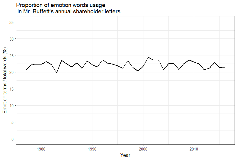
Emotion words in the annual shareholder letters accounted for approximately 20% – 25% of the total words count (excluding stop words and numbers). The median emotion count was ~22% of the total words count.

Depicting distribution of emotion words usage

### pull emotion words and aggregate by year and emotion terms
emotions <- letters %>% 
  unnest_tokens(word, text) %>%                           
  anti_join(stop_words, by = "word") %>%                  
  filter(!grepl('[0-9]', word)) %>%
  left_join(get_sentiments("nrc"), by = "word") %>%
  filter(!(sentiment == "negative" | sentiment == "positive")) %>%
  group_by(year, sentiment) %>%
  summarize( freq = n()) %>%
  mutate(percent=round(freq/sum(freq)*100)) %>%
  select(-freq) %>%
  ungroup()
### need to convert the data structure to a wide format
emo_box = emotions %>%
spread(sentiment, percent, fill=0) %>%
ungroup()
### color scheme for the box plots (This step is optional)
cols  <- colorRampPalette(brewer.pal(7, "Set3"), alpha=TRUE)(8)
boxplot2(emo_box[,c(2:9)], col=cols, lty=1, shrink=0.8, textcolor="red",        xlab="Emotion Terms", ylab="Emotion words count (%)", main="Distribution of emotion words count in annual shareholder letters (1978 - 2016")

Which gives this plot:

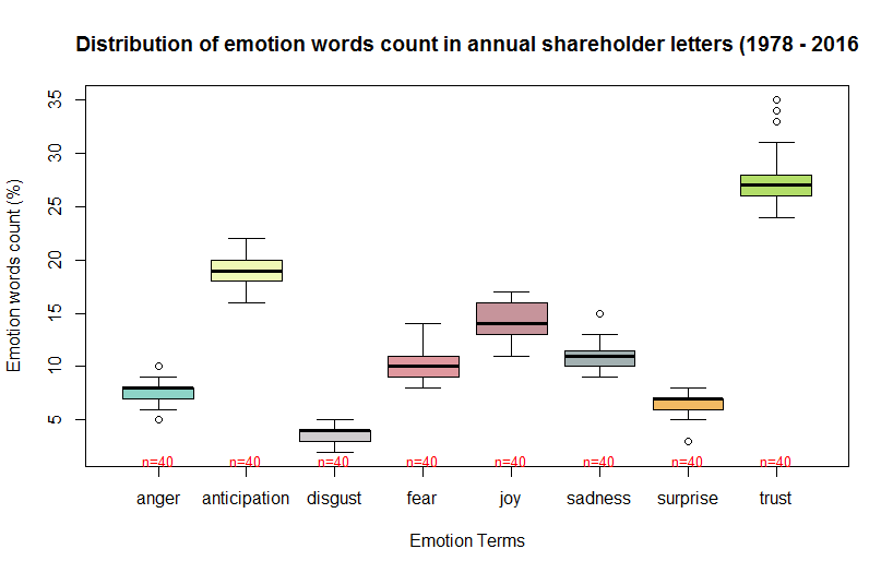
Terms for all eight emotions types were expressed albeit at variable rates. Looking at the box plot, anger, sadness, surprise and trust showed outliers. Besides, anger, disgust and surprise were skewed to the left, whereas Joy was skewed to the right. The n= below each box plot indicates the number of observations that contributed to the distribution of the box plot above it.

Emotion words usage over time

## yearly line chart
ggplot(emotions, aes(x=year, y=percent, color=sentiment, group=sentiment)) +
geom_line(size=1) +
geom_point(size=0.5) +
xlab("Year") +
  ylab("Emotion words count (%)") +
  ggtitle("Emotion words expressed in Mr. Buffett's \n annual shareholder letters")

Gives this plot:

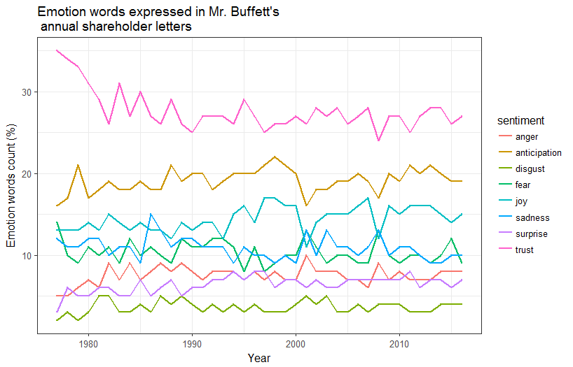
Clearly emotion terms referring to trust and anticipation were expressed consistently higher than the other emotion terms in all of the annual shareholder letters. Emotion terms referring to disgust, anger and surprise were expressed consistently lower than the other emotion terms at almost all time points.

Average emotion words expression using bar charts with error bars

### calculate overall averages and standard deviations for each emotion term
overall_mean_sd <- emotions %>%
     group_by(sentiment) %>%
     summarize(overall_mean=mean(percent), sd=sd(percent))
### draw a bar graph with error bars
ggplot(overall_mean_sd, aes(x = reorder(sentiment, -overall_mean), y=overall_mean)) +
     geom_bar(stat="identity", fill="darkgreen", alpha=0.7) + 
     geom_errorbar(aes(ymin=overall_mean-sd, ymax=overall_mean+sd), width=0.2,position=position_dodge(.9)) +
     xlab("Emotion Terms") +
     ylab("Emotion words count (%)") +
     ggtitle("Emotion words expressed in Mr. Buffett's \n annual shareholder letters (1977 – 2016)") + 
     theme(axis.text.x=element_text(angle=45, hjust=1)) +
     coord_flip( )

Which gives this plot:

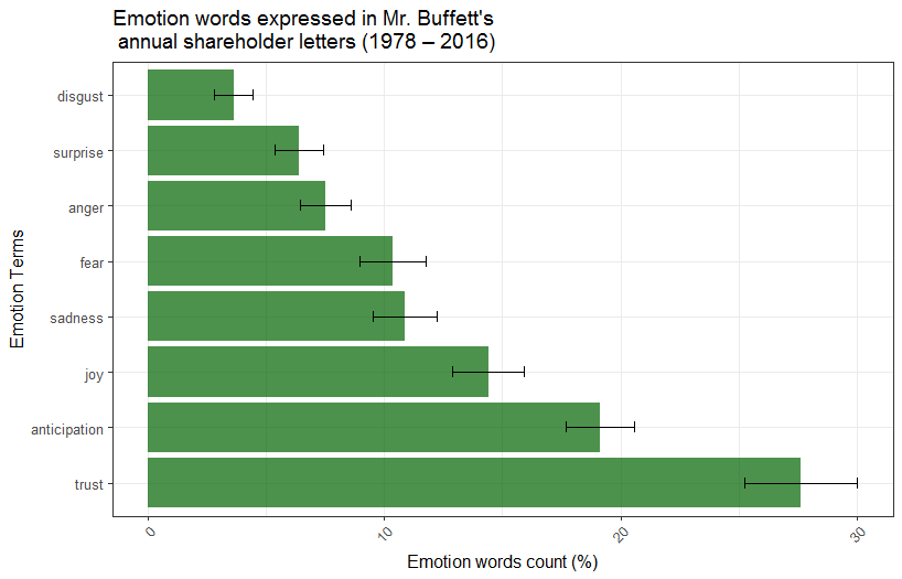
Emotion words referring to trust, anticipation and joy were over-represented and accounted on average for approximately 60% of all emotion words in all shareholder letters. On the other hand, disgust, surprise and anger were the least expressed emotion terms and accounted on average for approximately 18% of all emotion terms in all shareholder letters.

Emotion terms usage over time compared to 40-years averages

For the figure below, the 40-year averages of each emotion terms shown in the above bar chart were subtracted from the yearly percent emotions for any given year. The results were showing higher or lower than average emotion expression levels for the respective years.

## Hi / Low plots compared to the 40-years average
emotions_diff <- emotions  %>%
     left_join(overall_mean_sd, by="sentiment") %>%
     mutate(difference=percent-overall_mean)

ggplot(emotions_diff, aes(x=year, y=difference, colour=difference>0)) +
geom_segment(aes(x=year, xend=year, y=0, yend=difference),
size=1.1, alpha=0.8) +
geom_point(size=1.0) +
xlab("Emotion Terms") +
     ylab("Net emotion words count (%)") +
     ggtitle("Emotion words expressed in Mr. Buffett's \n annual shareholder letters (1977 - 2016)") + 
theme(legend.position="none") +
facet_wrap(~sentiment, ncol=4)

Gives this plot:

Red lines show lower than the 40-year average emotion expression levels, while blue lines indicate higher than the 40-year average emotion expression levels for the respective years.

Concluding Remarks

Excluding stop words and numbers, approximately 1 in 4 words in the annual shareholder letters represented emotion terms. Clearly emotion terms referring to trust, anticipation and joy accounted for approximately 60% of all emotion terms. There were also very limited emotions of fear (approximately 1 in 10 emotion terms). In conclusion, R offers several packages and functions for the evaluation and analyses of emotions words in textual data, as well as visualization and presentation of analysis results. Some of those packages and functions have been illustrated in this post. Hopefully, you find this post and analyses and visualization examples helpful.