
R does calculus without any extra packages. The stats package that loads with every session has D() and deriv() for symbolic derivatives, integrate() for definite integrals, and uniroot() and optimize() for finding where a function hits zero or reaches its maximum. I wanted to see how far those built-in tools go on real data instead of textbook functions, so every step below answers a question the raw numbers can’t.
The data is Theoph, which ships with R in the datasets package (documentation). Twelve people took a single oral dose of theophylline, an asthma drug, and had their blood concentration measured at 11 time points over the next 24 hours. The derivative of that concentration curve gives the time of the peak, and its integral, the area under the curve (AUC), gives the total exposure to the drug. Everything below runs on R 4.6.1, with dplyr, purrr and ggplot2 for data handling and figures.
How do I take a derivative in R?
Use D(): give it an expression and the name of the variable, and it returns the derivative as a new expression. deriv() does the same work but hands back a function that computes the value and the derivative (the gradient) together. This block runs on its own:
# Derivative of x^2 * exp(-x) with respect to x
D(quote(x^2 * exp(-x)), "x")
## 2 * x * exp(-x) - x^2 * exp(-x)
# Second derivative: apply D() to the result
D(D(quote(x^2 * exp(-x)), "x"), "x")
## 2 * exp(-x) - 2 * x * exp(-x) - (2 * x * exp(-x) - x^2 * exp(-x))
# deriv() returns a function; the gradient rides along as an attribute
g <- deriv(~ x^2 * exp(-x), "x", function.arg = TRUE)
g(1)
## [1] 0.3678794
## attr(,"gradient")
##              x
## [1,] 0.3678794
D() knows arithmetic, powers, exp(), log(), sqrt(), the trig functions, pnorm(), dnorm(), gamma() and a few more (?deriv has the full list). It does not simplify its answer, so expressions grow quickly with each derivative. If you want tidier output, the Deriv package does the same job and simplifies as it goes.
Fit a curve to the drug data
I start with subject 1. The standard model for a single oral dose is the one-compartment model: the drug is absorbed into the blood at rate ka, eliminated at rate ke, and Cl is the clearance.
$$C(t) = \frac{\text{Dose} \cdot k_e k_a}{Cl (k_a – k_e)} \left(e^{-k_e t} – e^{-k_a t}\right)$$
R has this model built in as SSfol(), a self-starting model, so nls() fits it without starting values. SSfol() estimates the three parameters on the log scale, which is why I exponentiate the coefficients.
library(dplyr)
library(purrr)
library(ggplot2)

theoph <- as_tibble(Theoph) |> mutate(Subject = as.character(Subject))
s1 <- theoph |> filter(Subject == "1")

fit1 <- nls(conc ~ SSfol(Dose, Time, lKe, lKa, lCl), data = s1)
pars <- exp(coef(fit1))
pars
##        lKe        lKa        lCl
## 0.05395450 1.77741701 0.01992348
For subject 1 the drug is absorbed at 1.78 per hour and eliminated at 0.054 per hour, a half-life of log(2) / ke = 12.8 hours. To use the fitted curve with D() and integrate(), I write it once as an expression and build a function from it:
conc_expr <- quote(dose * ke * ka / (Cl * (ka - ke)) * (exp(-ke * t) - exp(-ka * t)))
vals <- list(dose = s1$Dose[1], ke = pars[["lKe"]], ka = pars[["lKa"]], Cl = pars[["lCl"]])
conc_fun <- function(t) eval(conc_expr, c(list(t = t), vals))

conc_fun(c(1, 6, 24))
## [1] 8.739356 8.122117 3.075422
When does the concentration peak?
At the peak the curve stops rising and starts to fall, so its derivative is zero there. D() writes the derivative and uniroot() finds where it crosses zero:
rate_expr <- D(conc_expr, "t")
rate_expr
## -(dose * ke * ka/(Cl * (ka - ke)) * (exp(-ke * t) * ke - exp(-ka *
##     t) * ka))
rate_fun <- function(t) eval(rate_expr, c(list(t = t), vals))

tmax <- uniroot(rate_fun, interval = c(0, 24))$root
tmax
## [1] 2.027764
conc_fun(tmax)
## [1] 9.758291
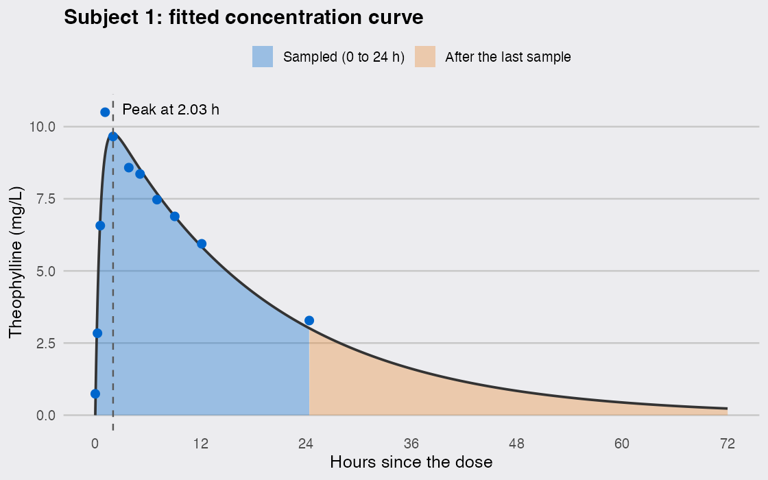
Subject 1 peaks 2.03 hours after the dose, at 9.76 mg/L. That is later and lower than the single highest sample (10.5 mg/L at 1.12 hours), because the fitted curve smooths over measurement noise instead of passing through every point. Two quick checks give the same peak. Setting the derivative to zero by hand gives tmax = log(ka / ke) / (ka – ke), and optimize() finds the maximum without using a derivative at all:
with(vals, log(ka / ke) / (ka - ke))
## [1] 2.027764
optimize(conc_fun, interval = c(0, 24), maximum = TRUE)$maximum
## [1] 2.027779
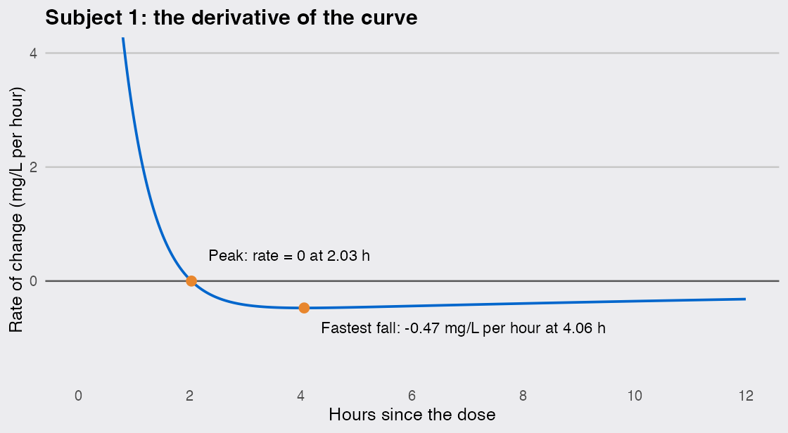
The derivative also says how fast the drug leaves the blood. Applying D() a second time gives the curvature, which is zero where the concentration falls fastest:
curv_expr <- D(rate_expr, "t")
curv_fun <- function(t) eval(curv_expr, c(list(t = t), vals))

t_fast <- uniroot(curv_fun, interval = c(tmax, 24))$root
c(t_fast = t_fast, two_tmax = 2 * tmax, rate = rate_fun(t_fast))
##     t_fast   two_tmax       rate
##  4.0555328  4.0555271 -0.4719398
The concentration falls fastest at 4.06 hours, by 0.47 mg/L per hour, and that is exactly twice the peak time. It is not a coincidence of this subject. Setting the second derivative of the model to zero gives the same relationship for any absorption and elimination rates:
$$t_{\text{fastest}} = \frac{2 \log(k_a / k_e)}{k_a – k_e} = 2 t_{\max}$$
Here is the derivative over the first 12 hours. The dsp_theme lines at the top of the chunk give the gray look used in all three figures; copy them if you like it.
dsp_colors <- c("#0066CC", "#E8862D", "#159A6C", "#7D5BD6",
                "#D64580", "#2AA9B8", "#C9A227")
dsp_theme <- theme_minimal(base_size = 13) +
  theme(plot.background    = element_rect(fill = "#ECECEF", color = NA),
        panel.background   = element_rect(fill = "#ECECEF", color = NA),
        panel.grid.minor   = element_blank(),
        panel.grid.major.x = element_blank(),
        panel.grid.major.y = element_line(color = "grey78"),
        axis.ticks         = element_blank(),
        plot.title         = element_text(face = "bold"),
        strip.text         = element_text(face = "bold"))

rates <- tibble(Time = seq(0, 12, by = 0.02), rate = rate_fun(Time))

ggplot(rates, aes(Time, rate)) +
  geom_hline(yintercept = 0, color = "grey35") +
  geom_line(linewidth = 0.9, color = dsp_colors[1]) +
  annotate("point", x = c(tmax, t_fast), y = c(0, rate_fun(t_fast)),
           color = dsp_colors[2], size = 3) +
  annotate("text", x = tmax + 0.3, y = 0.45, hjust = 0, size = 4,
           label = sprintf("Peak: rate = 0 at %.2f h", tmax)) +
  annotate("text", x = t_fast + 0.3, y = rate_fun(t_fast) - 0.35, hjust = 0, size = 4,
           label = sprintf("Fastest fall: %.2f mg/L per hour at %.2f h",
                           rate_fun(t_fast), t_fast)) +
  scale_x_continuous(breaks = seq(0, 12, 2)) +
  coord_cartesian(ylim = c(-1.5, 4)) +
  labs(x = "Hours since the dose", y = "Rate of change (mg/L per hour)",
       title = "Subject 1: the derivative of the curve") +
  dsp_theme
If your curve comes from a spline or a simulation, there is no formula for D() to read. A numerical derivative does the same job, and the numDeriv package agrees with D() here:
numDeriv::grad(conc_fun, 3)
## [1] -0.4187882
rate_fun(3)
## [1] -0.4187882
How do I integrate a function in R?
Use integrate() with the function and the two limits, and write Inf for an open-ended limit. The function has to take a vector and return a vector of the same length. If yours doesn’t, wrap it in Vectorize(), or integrate() stops with "evaluation of function gave a result of wrong length". This block runs on its own:
f <- function(x) x^2 * exp(-x)
integrate(f, lower = 0, upper = Inf)
## 2 with absolute error < 7.1e-05
# A function that ignores x returns one value, not a vector
integrate(Vectorize(function(x) 1), lower = 0, upper = 1)
## 1 with absolute error < 1.1e-14
For the drug curve, the integral from zero to infinity is the total exposure, AUC, in mg·h/L:
auc_inf <- integrate(conc_fun, lower = 0, upper = Inf)
auc_inf
## 201.772 with absolute error < 0.015
vals$dose / vals$Cl
## [1] 201.772
The second line is a check. Integrating the model by hand gives AUC = Dose / Cl exactly, and the two differ by about one part in 150 million.
You don’t need a model to get an AUC from data. The trapezoid rule joins the samples with straight lines and adds up the areas underneath, which is one line of R:
trapezoid <- function(x, y) sum(diff(x) * (head(y, -1) + tail(y, -1)) / 2)

t_last <- max(s1$Time)
auc_trap <- trapezoid(s1$Time, s1$conc)
auc_model_last <- integrate(conc_fun, lower = 0, upper = t_last)$value
auc_tail <- integrate(conc_fun, lower = t_last, upper = Inf)$value

c(trapezoid = auc_trap, model_to_last = auc_model_last, after_last = auc_tail)
##     trapezoid model_to_last    after_last
##     148.92305     145.89836      55.87367
The trapezoid area up to the last sample at 24.37 hours is 148.9, a little more than the model’s 145.9. Part of the gap is that a falling, convex curve sags below the straight lines between samples, so the trapezoids overshoot. The bigger number is the tail: 55.9 mg·h/L, or 27.7% of subject 1’s total exposure, arrives after the last blood draw.
curve_df <- tibble(Time = seq(0, 72, by = 0.05), conc = conc_fun(Time)) |>
  mutate(part = factor(if_else(Time <= t_last, "Sampled (0 to 24 h)", "After the last sample"),
                       levels = c("Sampled (0 to 24 h)", "After the last sample")))

ggplot(curve_df, aes(Time, conc)) +
  geom_area(aes(fill = part), alpha = 0.35) +
  geom_line(linewidth = 0.9, color = "grey20") +
  geom_point(data = s1, color = dsp_colors[1], size = 2.6) +
  geom_vline(xintercept = tmax, linetype = "dashed", color = "grey35") +
  annotate("text", x = tmax + 1, y = 10.6, hjust = 0, size = 4,
           label = sprintf("Peak at %.2f h", tmax)) +
  scale_fill_manual(values = dsp_colors[1:2], name = NULL) +
  scale_x_continuous(breaks = seq(0, 72, 12)) +
  labs(x = "Hours since the dose", y = "Theophylline (mg/L)",
       title = "Subject 1: fitted concentration curve") +
  dsp_theme +
  theme(legend.position = "top")
How much exposure does a 24-hour study miss?
Next I repeat the fit and the integrals for all 12 subjects. split() makes one data frame per subject and map() runs the same steps on each:
by_subject <- theoph |>
  split(~ Subject) |>
  map(function(d) {
    p <- exp(coef(nls(conc ~ SSfol(Dose, Time, lKe, lKa, lCl), data = d)))
    v <- list(dose = d$Dose[1], ke = p[["lKe"]], ka = p[["lKa"]], Cl = p[["lCl"]])
    f <- function(t) eval(conc_expr, c(list(t = t), v))
    tibble(half_life = log(2) / v$ke,
           auc_trap  = trapezoid(d$Time, d$conc),
           auc_inf   = integrate(f, 0, Inf)$value,
           auc_tail  = integrate(f, max(d$Time), Inf)$value)
  }) |>
  list_rbind(names_to = "Subject") |>
  mutate(pct_after_24h = 100 * auc_tail / auc_inf,
         pct_covered   = 100 * auc_trap / auc_inf)

by_subject |>
  arrange(desc(pct_after_24h)) |>
  mutate(across(where(is.numeric), \(x) round(x, 1)))
## # A tibble: 12 × 7
##    Subject half_life auc_trap auc_inf auc_tail pct_after_24h pct_covered
##    <chr>       <dbl>    <dbl>   <dbl>    <dbl>         <dbl>       <dbl>
##  1 1            12.8    149.    202.      55.9          27.7        73.8
##  2 10            9.4    138.    170.      32.9          19.4        81.6
##  3 3             8.5     99.3   114.      16.6          14.5        86.7
##  4 4             7.9    107.    118.      14.7          12.5        90.8
##  5 5             7.8    121.    134.      16.6          12.4        90.3
##  6 9             8       86.3    94.8     11.5          12.2        91
##  7 8             7.5     88.6    97.5     11.4          11.7        90.8
##  8 6             7       73.8    78.2      8            10.2        94.3
##  9 7             6.8     90.8    95.9      9.5           9.9        94.6
## 10 11            7.1     80.1    85.9      8.3           9.7        93.2
## 11 12            6.6    120     126.      11.3           8.9        95.1
## 12 2             6.8     91.5    98.3      8.8           8.9        93.1
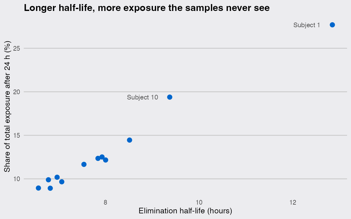
The share of exposure that comes after the last sample runs from 8.9% (subject 2) to 27.7% (subject 1), with a median of 11.9%. What decides it is the half-life: the two track each other with a correlation of 0.99. A good back-of-the-envelope figure is 0.5^(24 / half-life), the part of the dose the body hasn’t cleared yet at 24 hours. With an 8-hour half-life that is 0.5³ = 12.5%; for subject 1’s 12.8 hours it is 27.4%.
This matters outside a tutorial. The European Medicines Agency’s bioequivalence guideline (section 4.1.4) asks for a sampling schedule where AUC(0-t), the area measured up to the last sample, covers at least 80% of AUC(0-∞). Measured against the fitted curves, the trapezoid AUC here covers between 73.8% and 95.1%. Subject 1 falls short at 73.8%, and subject 10 clears the bar by only 1.6 points.
ggplot(by_subject, aes(half_life, pct_after_24h)) +
  geom_point(color = dsp_colors[1], size = 3.2) +
  geom_text(data = filter(by_subject, half_life > 9),
            aes(label = paste("Subject", Subject)),
            nudge_x = -0.25, hjust = 1, size = 3.8, color = "grey30") +
  labs(x = "Elimination half-life (hours)",
       y = "Share of total exposure after 24 h (%)",
       title = "Longer half-life, more exposure the samples never see") +
  dsp_theme
Why does integrate() return zero for a large upper limit?
Because it sampled the function only where the function is zero. Over a finite range, integrate() starts by evaluating the function at 21 points spread across the interval, then refines wherever its error estimate says it should. If the interval is so wide that every one of those points lands where the curve is practically zero, the error estimate is tiny too, and it stops with a confident wrong answer. Here is what happens when I replace Inf with "a very long time":
integrate(conc_fun, lower = 0, upper = Inf)
## 201.772 with absolute error < 0.015
integrate(conc_fun, lower = 0, upper = 1e5)
## 201.772 with absolute error < 3.8e-06
integrate(conc_fun, lower = 0, upper = 1e6)
## 1.190449e-21 with absolute error < 2.4e-21
Up to 100,000 hours the answer is right. At a million hours it is 1.2e-21, with an error estimate just as small and no warning. With that upper limit, the sample point closest to zero sits about 2,170 hours after the dose, long after the drug is gone. The help page says it plainly: "When integrating over infinite intervals do so explicitly, rather than just using a large number as the endpoint." So pass Inf, or split the range at a point you know is past the action, as in integrate(conc_fun, 0, 72)$value + integrate(conc_fun, 72, Inf)$value.
The calculus toolkit in base R
D(expr, "x")returns the derivative of an expression; apply it again for the second derivative.deriv()returns a function that computes the value and its gradient.uniroot(f, interval)finds where a function is zero, such as where a derivative vanishes.optimize(f, interval, maximum = TRUE)finds a maximum (or minimum) directly.integrate(f, lower, upper)computes a definite integral, andupper = Infworks; passInfrather than a large number.- For data without a model, the trapezoid rule is one line, and
numDeriv::grad()gives numerical derivatives of any function.
