Outliers Detection and Intervention Analysis

In my previous tutorial Arima Models and Intervention Analysis we took advantage of the strucchange package to identify and date time series level shifts structural changes. Based on that, we were able to define ARIMA models with improved AIC metrics. Furthermore, the attentive analysis of the ACF/PACF plots highlighted the presence of seasonal patterns. In this tutorial we will investigate another flavour of intervention variable, the transient change. We will take advantage of two fundamental packages for the purpose:

* tsoutliers
* TSA

Specifically, we will compare results obtained by modeling the transient change.

Outliers Analysis

Outliers detection relates with intervention analysis as the latter can be argued as a special case of the former one. A basic list of intervention variable is:

* step response intervention
* pulse response intervention

A basic list of outliers is:

* Additive Outliers
* Level Shifts
* Transient Change 
* Innovation Outliers
* Seasonal Level Shifts

An Additive Outlier (AO) represents an isolated spike.
A Level Shift (LS) represents an abrupt change in the mean level and it may be seasonal (Seasonal Level Shift, SLS) or not.
A Transient Change (TC) represents a spike that takes a few periods to disappear.
An Intervention Outlier (IO) represents a shock in the innovations of the model.

Pre-specified outliers are able to satisfactorily describe the dynamic pattern of untypical effects and can be captured by means of intervention variables.

Intervention Analysis – Common Models

A short introduction of the very basic common models of functions useful for intervention analysis follows.

Step function

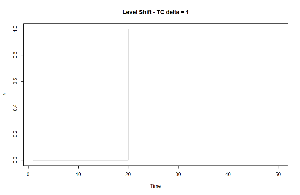
The step function is useful to represent level shift outliers.

$$
\begin{equation}
\begin{aligned}
S_{T}(t) &=\left\{
\begin{array}{@{}ll@{}}
0 & \text{if}\ t < T \\
1 & \text{otherwise}\
\end{array} \right.
\end{aligned}
\end{equation}
$$

It can be thought as a special case of the transient change intervention model with delta = 1 (see ahead the transient change model). We can represent it with the help of the filter() function as follows. .

tc <- rep(0, 50)
tc[20] <- 1
ls <- filter(tc, filter = 1, method = "recursive")
plot(ls, main = "Level Shift - TC delta = 1", type = "s")

By adding up two step functions at different lags, it is possible to represent additive outliers or transitory level shifts, as we will see soon.

Pulse function

The pulse function is useful to represent additive outliers.

$$
\begin{equation}
\begin{aligned}
P_{T}(t) = S_{T}(t)\ -\ S_{T}(t-1)
\end{aligned}
\end{equation}
$$

It can be thought as a special case of the transient change intervention model with delta = 0 (see ahead the transient change model). We can graphically represent it with the help of the filter() function as herein shown.

ao <- filter(tc, filter = 0, method = "recursive")
plot(ao, main = "Additive Outlier - TC delta = 0", type = "s")

Level Shift function

The level shift function is useful to represent level shift outliers. It can be modeled in terms of step function with magnitude equal to the omega parameter.

$$
\begin{equation}
\begin{aligned}
m(t) = \omega S_{T}(t)
\end{aligned}
\end{equation}
$$

The graphical representation is the same of the step function with magnitude equal to the omega parameter of the formula above.

Transient change function

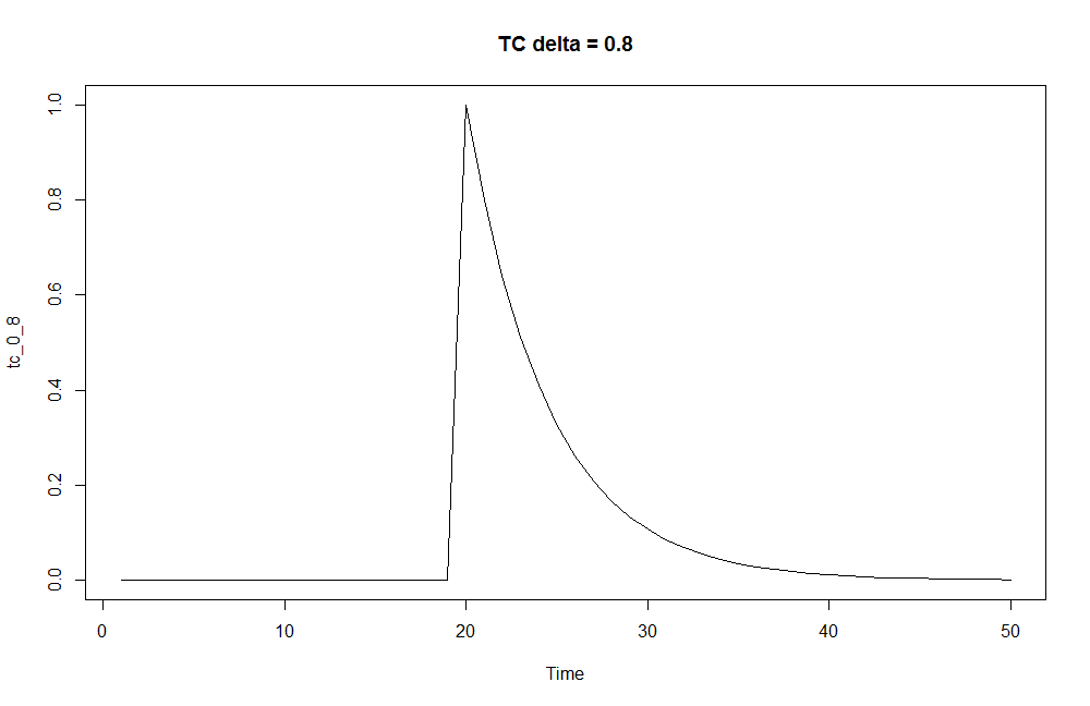
The transient change function is useful to represent transient change outliers.

$$
\begin{equation}
\begin{aligned}
\ C(t) = \dfrac{\omega B}{1 – \delta B} P_{T}(t)
\end{aligned}
\end{equation}
$$

We can graphically represent it by the help of the filter() function as herein shown. Two delta values are considered to show how the transient change varies accordingly.

tc_0_4 <- filter(tc, filter = 0.4, method = "recursive")
tc_0_8 <- filter(tc, filter = 0.8, method = "recursive")
plot(tc_0_4, main = "TC delta = 0.4")
plot(tc_0_8, main = "TC delta = 0.8")

Packages

suppressPackageStartupMessages(library(tsoutliers))
suppressPackageStartupMessages(library(TSA))
suppressPackageStartupMessages(library(lmtest))
suppressPackageStartupMessages(library(astsa))

Analysis

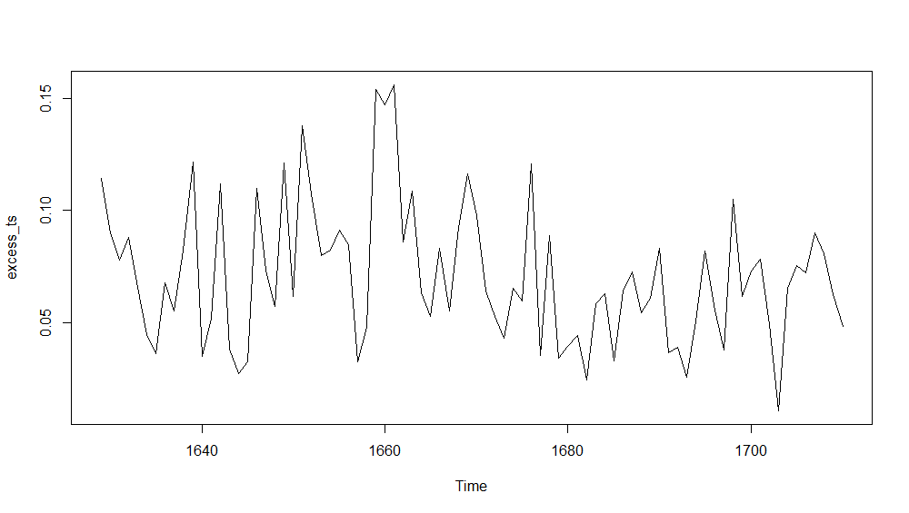
In the following, I will analyse the sex ratio at birth as based on the Arbuthnot dataset which provides information of male and female births in London from year 1639 to 1710. As done in ref. [1], a metric representing the fractional excess of boys births versus girls is defined as:

$$
\begin{equation}
\begin{aligned}
\dfrac{(Boys – Girls)}{Girls}
\end{aligned}
\end{equation}
$$

url <- "https://www.openintro.org/stat/data/arbuthnot.csv"
abhutondot <- read.csv(url, header=TRUE)

boys_ts <- ts(abhutondot$boys, frequency=1, start = abhutondot$year[1])
girls_ts <- ts(abhutondot$girls, frequency=1, start = abhutondot$year[1])

delta_ts <- boys_ts - girls_ts
excess_ts <- delta_ts/girls_ts
plot(excess_ts)

Gives this plot.

With the help of the tso() function within tsoutliers package, we identify if any outliers are present in our excess_ts time series.

outliers_excess_ts <- tso(excess_ts, types = c("TC", "AO", "LS", "IO", "SLS"))
outliers_excess_ts
Series: excess_ts 
Regression with ARIMA(0,0,0) errors 

Coefficients:
      intercept    TC31
         0.0665  0.1049
s.e.     0.0031  0.0199

sigma^2 estimated as 0.0007378:  log likelihood=180.34
AIC=-354.69   AICc=-354.38   BIC=-347.47

Outliers:
  type ind time coefhat tstat
1   TC  31 1659  0.1049 5.283

A transient change outlier occurring on year 1659 was identified. We can inspect graphically the results too.

plot(outliers_excess_ts)

Gives this plot.

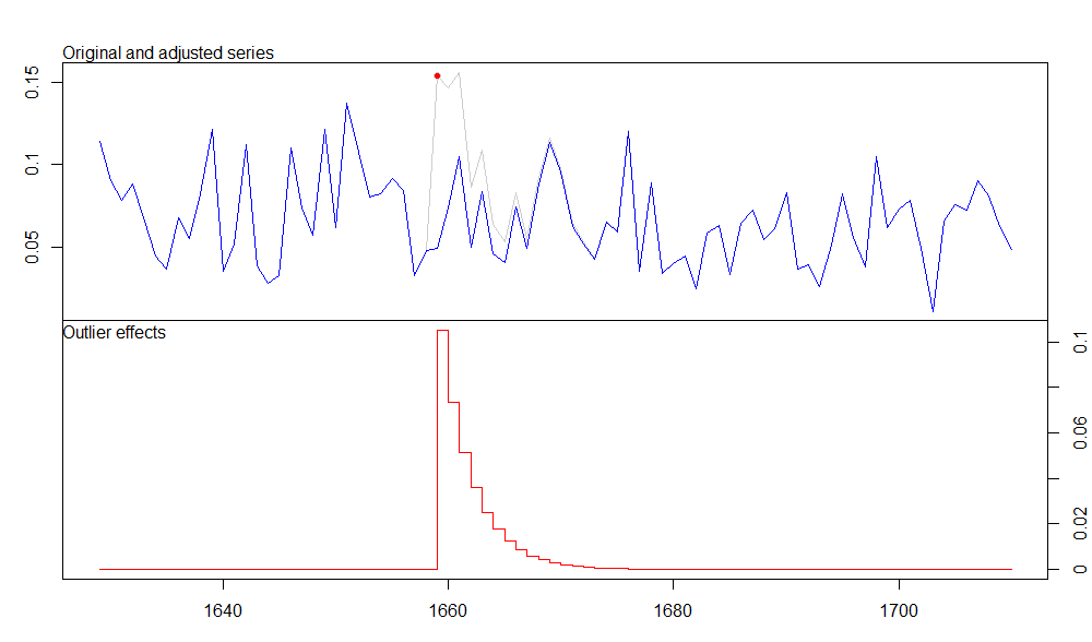
We found an outlier of Transient Change flavour occurring on year 1659. Specific details are herein shown.

outliers_excess_ts$outliers
  type ind time   coefhat   tstat
1   TC  31 1659 0.1049228 5.28339

# time index where the outliers have been detected
(outliers_idx <- outliers_excess_ts$outliers$ind)
[1] 31

# calendar years where the outliers have been detected 
outliers_excess_ts$outliers$time
[1] 1659

We now want to evaluate the effect of such transient change, comparing the original time series under analysis with the same without such transient change.

#length of our time series
n <- length(excess_ts)

# transient change outlier at the same time index as found for our time series
mo_tc <- outliers("TC", outliers_idx)

# transient change effect data is stored into a one-column matrix, tc
tc <- outliers.effects(mo_tc, n)
             TC31
 [1,] 0.000000e+00
 [2,] 0.000000e+00
 [3,] 0.000000e+00
 [4,] 0.000000e+00
 [5,] 0.000000e+00
 [6,] 0.000000e+00
 [7,] 0.000000e+00
 [8,] 0.000000e+00
 [9,] 0.000000e+00
[10,] 0.000000e+00
...

The “coefhat” named data frame stores the coefficient used as multiplier for our transient change tc data matrix.

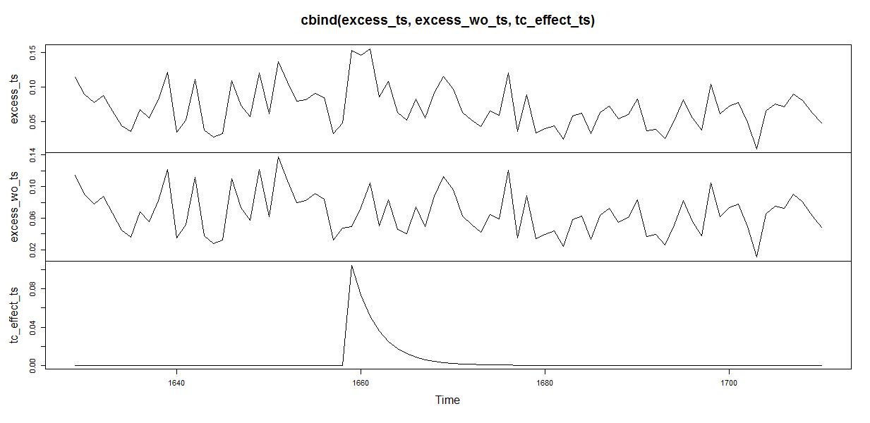
# converting to a number
coefhat <- as.numeric(outliers_excess_ts$outliers["coefhat"])

# obtaining the transient change data with same magnitude as determined by the tso() function
tc_effect <- coefhat*tc

# definining a time series for the transient change data
tc_effect_ts <- ts(tc_effect, frequency = frequency(excess_ts), start = start(excess_ts))

# subtracting the transient change intervention to the original time series, obtaining a time series without the transient change effect
excess_wo_ts <- excess_ts - tc_effect_ts

# plot of the original, without intervention and transient change time series 
plot(cbind(excess_ts, excess_wo_ts, tc_effect_ts))

Gives this plot.

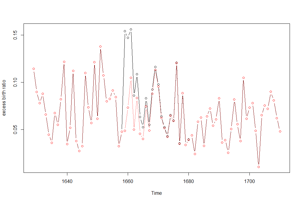
We can further highlight the difference between the original time series and same time series without the transient change effect.

plot(excess_ts, type ='b', ylab = "excess birth ratio")
lines(excess_wo_ts, col = 'red', lty = 3, type ='b')

Gives this plot.

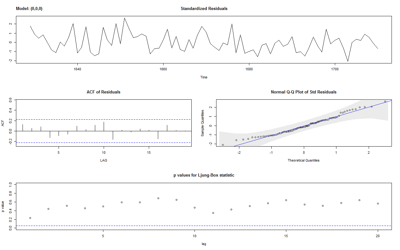
A quick check on the residuals of the time series without the transient change effect confirms validity of the ARIMA(0,0,0) model.

sarima(excess_wo_ts, p=0, d=0, q=0)

Gives this plot.

Now, we implement a similar representation of the transient change outlier by taking advantage of the arimax() function within the TSA package. The arimax() function requires to specify some ARMA parameters, and that is done by capturing the seasonality as discussed in ref. [1]. Further, the transient change is specified by means of xtransf and transfer input parameters. The xtransf parameter is a matrix with each column containing a covariate that affects the time series response in terms of an ARMA filter of order (p,q). For our scenario, it provides a value equal to 1 at the outliers time index and zero at others. The transfer parameter is a list consisting of the ARMA orders for each transfer covariate. For our scenario, we specify an AR order equal to 1.

arimax_model <- arimax(excess_ts,
                       order = c(0,0,0),
                       seasonal = list(order = c(1,0,0), period = 10),
                       xtransf = data.frame(I1 = (1*(seq(excess_ts) == outliers_idx))),                                                                                      
                       transfer = list(c(1,0)),
                       method='ML')

summary(arimax_model)
Call:
arimax(x = excess_ts, order = c(0, 0, 0), seasonal = list(order = c(1, 0, 0), 
    period = 10), method = "ML", xtransf = data.frame(I1 = (1 * (seq(excess_ts) == 
    outliers_idx))), transfer = list(c(1, 0)))

Coefficients:
        sar1  intercept  I1-AR1  I1-MA0
      0.2373     0.0668  0.7601  0.0794
s.e.  0.1199     0.0039  0.0896  0.0220

sigma^2 estimated as 0.0006825:  log likelihood = 182.24,  aic = -356.48

Training set error measures:
                        ME      RMSE        MAE       MPE     MAPE      MASE      ACF1
Training set -0.0001754497 0.0261243 0.02163487 -20.98443 42.09192 0.7459687 0.1429339

The significance of the coefficients is then verified.

coeftest(arimax_model)
z test of coefficients:

           Estimate Std. Error z value  Pr(>|z|)    
sar1      0.2372520  0.1199420  1.9781 0.0479224 *  
intercept 0.0667816  0.0038564 17.3173 < 2.2e-16 ***
I1-AR1    0.7600662  0.0895745  8.4853 < 2.2e-16 ***
I1-MA0    0.0794284  0.0219683  3.6156 0.0002997 ***
---
Signif. codes:  0 ‘***’ 0.001 ‘**’ 0.01 ‘*’ 0.05 ‘.’ 0.1 ‘ ’ 1

The model coefficients are all statistically significative. We remark that the resulting model shows a slight improved AIC result with respect the previous model. Further, both models show improved AIC values with respect previous tutorial discussed ARIMA models.

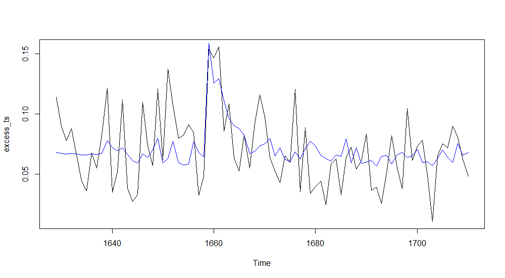
Let us plot the original time series against the fitted one.

plot(excess_ts)
lines(fitted(arimax_model), col = 'blue')

Gives this plot.

Considering the transient change model formula, we can elaborate a linear filter with the AR parameter as coefficient and the MA parameter to multiply the filter() function result.

# pulse intervention variable
int_var <- 1*(seq(excess_ts) == outliers_idx)

# transient change intervention variable obtained by filtering the pulse according to the
# definition of transient change and parameters obtained by the ARIMAX model 
tc_effect_arimax <- filter(int_var, filter = coef(arimax_model)["I1-AR1"], 
                          method = "rec", sides = 1) * coef(arimax_model)["I1-MA0"]

# defining the time series for the intervention effect
tc_effect_arimax_ts <- ts(tc_effect_arimax, frequency = frequency(excess_ts), start = start(excess_ts))

It is interesting to compare two transient change effects, as obtained by the arimax() and the tso() functions.

# comparing transient change effect resulting by ARIMAX (red) with the tso() one (blue)
plot(tc_effect_arimax_ts, col ='red', type='l', ylab = "transient change")
lines(tc_effect_ts, col ='blue', lty = 3)

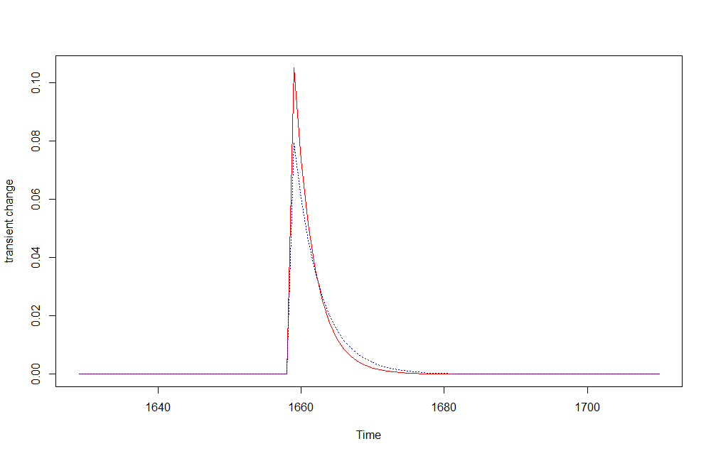
By eyeballing the plot above, they appear pretty close.

A quick check on the residuals of the time series without the transient change effect confirms the validity of the ARIMA(0,0,0)(1,0,0)[10] model.

excess_wo_arimax_ts <- excess_ts - tc_effect_arimax_ts 
sarima(excess_wo_arimax_ts, p=0, d=0, q=0, P=1, D=0, Q=0, S=10)

Gives this plot.

If you have any questions, please feel free to comment below.

References

[1] Arima Models and Intervention Analysis – DataScience+
[2] Time Series Analysis With Applications in R
[3] ARIMA Intervention Analysis – How to visualize the effect
[4] Detecting outliers in a time series