In my previous tutorial Structural Changes in Global Warming I introduced the strucchange package and some basic examples to date structural breaks in time series. In the present tutorial, I am going to show how dating structural changes (if any) and then Intervention Analysis can help in finding better ARIMA models. Dating structural changes consists in determining if there are any structural breaks in the time series data generating process, and, if so, their dates. Intervention analysis estimates the effect of an external or exogenous intervention on a time series. As an example of intervention, a permanent level shift, as we will see in this tutorial. In our scenario, the external or exogenous intervention is not known in advance, (or supposed to be known), it is inferred from the structural break we will identify.
The dataset considered for the analysis is the Arbuthnot dataset containing information of male and female births in London from year 1639 to 1710. Based on that, a metric representing the fractional excess of boys births versus girls is defined as:
$$
\begin{equation}
\begin{aligned}
\dfrac{(Boys – Girls)}{Girls}
\end{aligned}
\end{equation}
$$
The time series so defined is analyzed to determine candidate ARIMA models. The present tutorial is so organized. First, a brief exploratory analysis is carried on. Then, six ARIMA models are defined, analyzed and compared. Forecast of the time series under analysis is computed. Finally, a short historical background digression is introduced describing what was happening in England on 17-th century and citing studies on the matter of sex ratio at birth.
Packages
suppressPackageStartupMessages(library(ggplot2))
suppressPackageStartupMessages(library(forecast))
suppressPackageStartupMessages(library(astsa))
suppressPackageStartupMessages(library(lmtest))
suppressPackageStartupMessages(library(fUnitRoots))
suppressPackageStartupMessages(library(FitARMA))
suppressPackageStartupMessages(library(strucchange))
suppressPackageStartupMessages(library(reshape))
suppressPackageStartupMessages(library(Rmisc))
suppressPackageStartupMessages(library(fBasics))
Note: The fUnitRoots package is not any longer maintained by CRAN, however it can be installed from source available at the following link:
fUnitRoots version 3010.78 sources
Exploratory Analysis
Loading the Arbuthnot dataset and showing some basic metrics and plots.
url <- "https://www.openintro.org/stat/data/arbuthnot.csv"
abhutondot <- read.csv(url, header=TRUE)
nrow(abhutondot)
[1] 82
head(abhutondot)
        year    boys    girls
1	1629	5218	4683
2	1630	4858	4457
3	1631	4422	4102
4	1632	4994	4590
5	1633	5158	4839
6	1634	5035	4820
abhutondot_rs <- melt(abhutondot, id = c("year"))
head(abhutondot_rs)
  year variable value
1 1629     boys  5218
2 1630     boys  4858
3 1631     boys  4422
4 1632     boys  4994
5 1633     boys  5158
6 1634     boys  5035
tail(abhutondot_rs)
    year variable value
159 1705    girls  7779
160 1706    girls  7417
161 1707    girls  7687
162 1708    girls  7623
163 1709    girls  7380
164 1710    girls  7288
ggplot(data = abhutondot_rs, aes(x = year)) + geom_line(aes(y = value, colour = variable)) +
       scale_colour_manual(values = c("blue", "red"))
Gives this plot.

Boys births appear to be consistently greater than girls ones. Let us run a t.test to further verify if there is a true difference in the mean of the two groups as represented by boys and girls births.
t.test(value ~ variable, data = abhutondot_rs)
Welch Two Sample t-test

data:  value by variable
t = 1.4697, df = 161.77, p-value = 0.1436
alternative hypothesis: true difference in means is not equal to 0
95 percent confidence interval:
 -128.0016  872.9040
sample estimates:
 mean in group boys mean in group girls
           5907.098            5534.646
Based on the p-value, we cannot reject the null hypothesis that the true difference in means is equal to zero.
basicStats(abhutondot[-1])
                     boys         girls
nobs         8.200000e+01  8.200000e+01
NAs          0.000000e+00  0.000000e+00
Minimum      2.890000e+03  2.722000e+03
Maximum      8.426000e+03  7.779000e+03
1. Quartile  4.759250e+03  4.457000e+03
3. Quartile  7.576500e+03  7.150250e+03
Mean         5.907098e+03  5.534646e+03
Median       6.073000e+03  5.718000e+03
Sum          4.843820e+05  4.538410e+05
SE Mean      1.825161e+02  1.758222e+02
LCL Mean     5.543948e+03  5.184815e+03
UCL Mean     6.270247e+03  5.884477e+03
Variance     2.731595e+06  2.534902e+06
Stdev        1.652754e+03  1.592137e+03
Skewness    -2.139250e-01 -2.204720e-01
Kurtosis    -1.221721e+00 -1.250893e+00
p1 <- ggplot(data = abhutondot_rs, aes(x = variable, y = value)) + geom_boxplot()
p2 <- ggplot(data = abhutondot, aes(boys)) + geom_density()
p3 <- ggplot(data = abhutondot, aes(girls)) + geom_density()
multiplot(p1, p2, p3, cols = 3)
Gives this plot.
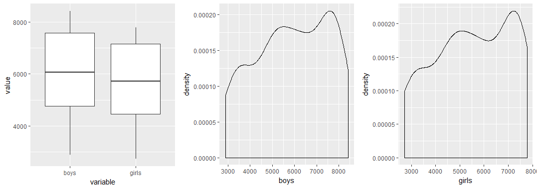
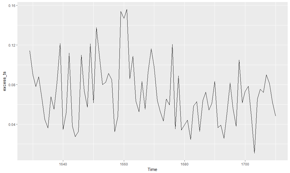
Let us define the time series to be analysed with frequency = 1 as data is collected yearly, see ref. [5] for details.
excess_frac <- (abhutondot$boys - abhutondot$girls)/abhutondot$girls
excess_ts <- ts(excess_frac, frequency = 1, start = abhutondot$year[1])
autoplot(excess_ts)
Gives this plot.
Basic statistics metrics are reported.
basicStats(excess_frac)
           excess_frac
nobs          82.000000
NAs            0.000000
Minimum        0.010673
Maximum        0.156075
1. Quartile    0.048469
3. Quartile    0.087510
Mean           0.070748
Median         0.064704
Sum            5.801343
SE Mean        0.003451
LCL Mean       0.063881
UCL Mean       0.077615
Variance       0.000977
Stdev          0.031254
Skewness       0.680042
Kurtosis       0.073620
Boys births were at least 1% higher than girls ones, reaching a top percentage excess equal to 15%.
Further, unit roots tests (run by urdfTest() within fUnitRoots package) show that we cannot reject the null hypothesis of unit root presence. See their test statistics compared with critical values below (see ref. [2] for details about the urdfTest() report).
urdftest_lag = floor(12*(length(excess_ts)/100)^0.25)
urdfTest(excess_ts, type = "nc", lags = urdftest_lag, doplot = FALSE)
Title:
 Augmented Dickey-Fuller Unit Root Test
Test Results:
  Test regression none
  Call:
  lm(formula = z.diff ~ z.lag.1 - 1 + z.diff.lag)

  Residuals:
        Min        1Q    Median        3Q       Max
  -0.052739 -0.018246 -0.002899  0.019396  0.069349

  Coefficients:
               Estimate Std. Error t value Pr(>|t|)
  z.lag.1      -0.01465    0.05027  -0.291 0.771802
  z.diff.lag1  -0.71838    0.13552  -5.301 1.87e-06 ***
  z.diff.lag2  -0.66917    0.16431  -4.073 0.000143 ***
  z.diff.lag3  -0.58640    0.18567  -3.158 0.002519 **
  z.diff.lag4  -0.56529    0.19688  -2.871 0.005700 **
  z.diff.lag5  -0.58489    0.20248  -2.889 0.005432 **
  z.diff.lag6  -0.60278    0.20075  -3.003 0.003944 **
  z.diff.lag7  -0.43509    0.20012  -2.174 0.033786 *
  z.diff.lag8  -0.28608    0.19283  -1.484 0.143335
  z.diff.lag9  -0.14212    0.18150  -0.783 0.436769
  z.diff.lag10  0.13232    0.15903   0.832 0.408801
  z.diff.lag11 -0.07234    0.12774  -0.566 0.573346
  ---
  Signif. codes:  0 ‘***’ 0.001 ‘**’ 0.01 ‘*’ 0.05 ‘.’ 0.1 ‘ ’ 1

  Residual standard error: 0.03026 on 58 degrees of freedom
  Multiple R-squared:  0.4638,	Adjusted R-squared:  0.3529
  F-statistic: 4.181 on 12 and 58 DF,  p-value: 0.0001034

  Value of test-statistic is: -0.2914
  Critical values for test statistics:
       1pct  5pct 10pct
  tau1 -2.6 -1.95 -1.61
urdfTest(excess_ts, type = "c", lags = urdftest_lag, doplot = FALSE)
Title:
 Augmented Dickey-Fuller Unit Root Test

Test Results:
  Test regression drift
  Call:
  lm(formula = z.diff ~ z.lag.1 + 1 + z.diff.lag)
  Residuals:
        Min        1Q    Median        3Q       Max
  -0.051868 -0.018870 -0.005227  0.019503  0.067936

  Coefficients:
               Estimate Std. Error t value Pr(>|t|)
  (Intercept)   0.02239    0.01789   1.251   0.2159
  z.lag.1      -0.31889    0.24824  -1.285   0.2041
  z.diff.lag1  -0.44287    0.25820  -1.715   0.0917 .
  z.diff.lag2  -0.40952    0.26418  -1.550   0.1266
  z.diff.lag3  -0.34933    0.26464  -1.320   0.1921
  z.diff.lag4  -0.35207    0.25966  -1.356   0.1805
  z.diff.lag5  -0.39863    0.25053  -1.591   0.1171
  z.diff.lag6  -0.44797    0.23498  -1.906   0.0616 .
  z.diff.lag7  -0.31103    0.22246  -1.398   0.1675
  z.diff.lag8  -0.19044    0.20656  -0.922   0.3604
  z.diff.lag9  -0.07128    0.18928  -0.377   0.7079
  z.diff.lag10  0.18023    0.16283   1.107   0.2730
  z.diff.lag11 -0.04154    0.12948  -0.321   0.7495
  ---
  Signif. codes:  0 ‘***’ 0.001 ‘**’ 0.01 ‘*’ 0.05 ‘.’ 0.1 ‘ ’ 1

  Residual standard error: 0.03012 on 57 degrees of freedom
  Multiple R-squared:  0.4781,	Adjusted R-squared:  0.3683
  F-statistic: 4.352 on 12 and 57 DF,  p-value: 6.962e-05

  Value of test-statistic is: -1.2846 0.8257

  Critical values for test statistics:
        1pct  5pct 10pct
  tau2 -3.51 -2.89 -2.58
  phi1  6.70  4.71  3.86
ACF and PACF plots are given.
par(mfrow=c(1,2))
acf(excess_ts)
pacf(excess_ts)
Gives this plot:
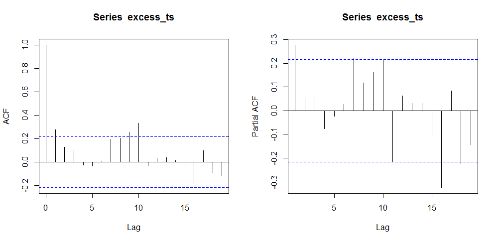
We observe the auto-correlation spike at lag = 10 beyond confidence region. That suggests the presence of a seasonal component with period = 10. Structural changes are now investigated. First let us verify if regression against a constant is significative for our time series.
summary(lm(excess_ts ~ 1))
Call:
lm(formula = excess_ts ~ 1)

Residuals:
      Min        1Q    Median        3Q       Max
-0.060075 -0.022279 -0.006044  0.016762  0.085327

Coefficients:
            Estimate Std. Error t value Pr(>|t|)
(Intercept) 0.070748   0.003451    20.5   <2e-16 ***
---
Signif. codes:  0 ‘***’ 0.001 ‘**’ 0.01 ‘*’ 0.05 ‘.’ 0.1 ‘ ’ 1

Residual standard error: 0.03125 on 81 degrees of freedom
The intercept is reported as significative. Let us see if there are any structural breaks.
(break_point <- breakpoints(excess_ts ~ 1))
	 Optimal 2-segment partition:

Call:
breakpoints.formula(formula = excess_ts ~ 1)
Breakpoints at observation number:
42
Corresponding to breakdates:
1670
plot(break_point)
Gives this plot.
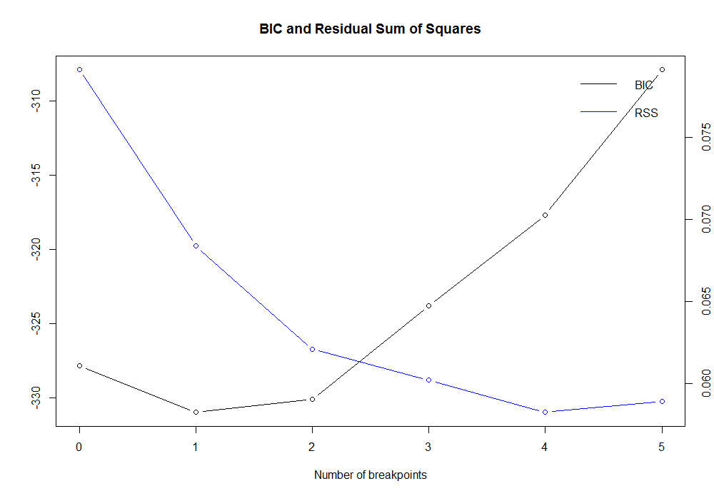
summary(break_point)
	 Optimal (m+1)-segment partition:
Call:
breakpoints.formula(formula = excess_ts ~ 1)
Breakpoints at observation number:
m = 1         42
m = 2   20    42
m = 3   20 35 48
m = 4   20 35    50 66
m = 5   17 30 42 56 69
Corresponding to breakdates:
m = 1             1670
m = 2   1648      1670
m = 3   1648 1663 1676
m = 4   1648 1663      1678 1694
m = 5   1645 1658 1670 1684 1697

Fit:
m   0          1          2          3          4          5
RSS    0.07912    0.06840    0.06210    0.06022    0.05826    0.05894
BIC -327.84807 -330.97945 -330.08081 -323.78985 -317.68933 -307.92410
The BIC minimum value is reached when m = 1, hence just one break point is determined corresponding to year 1670. Let us plot the original time series against its structural break and its confidence interval.
plot(excess_ts)
lines(fitted(break_point, breaks = 1), col = 4)
lines(confint(break_point, breaks = 1))
Gives this plot.

Boys vs girls sex ratio at birth changed from:
fitted(break_point)[1]
0.08190905
to:
fitted(breakpoint)[length(excess_ts)]
0.05902908
Running a t.test() to verify further the difference in mean is significative across the two time windows identified by the breakpoint date, year 1670.
break_date <- breakdates(break_point)
win_1 <- window(excess_ts, end = break_date)
win_2 <- window(excess_ts, start = break_date + 1)
t.test(win_1, win_2)
Welch Two Sample t-test
data:  win_1 and win_2
t = 3.5773, df = 70.961, p-value = 0.0006305
alternative hypothesis: true difference in means is not equal to 0
95 percent confidence interval:
 0.01012671 0.03563322
sample estimates:
 mean of x  mean of y
0.08190905 0.05902908
Based on reported p-value, we reject the null hypothesis that the true difference is equal to zero.
ARIMA Models
I am going to compare the following six ARIMA models (represented with the usual (p,d,q)(P,D,Q)[S] notation):
1. non seasonal (1,1,1), as determined by auto.arima() within forecast package
2. seasonal (1,0,0)(0,0,1)[10]
3. seasonal (1,0,0)(1,0,0)[10]
4. seasonal (0,0,0)(0,0,1)[10] with level shift regressor as intervention variable
5. seasonal (1,0,0)(0,0,1)[10] with level shift regressor as intervention variable
6. non seasonal (1,0,0) with level shift regressor as intervention variable
Here we go.
Model #1
The first model is determined by the auto.arima() function within the forecast package, using the options:
a. stepwise = FALSE, which allows for a more in-depth search of potential models
b. trace = TRUE, which allows to get a list of all the investigated models
Further, as default input to auto.arima() :
c. stationary = FALSE, so that models search is not restricted to stationary models
d. seasonal = TRUE, so that models search is not restricted to non seasonal models
(model_1 <- auto.arima(excess_ts, stepwise = FALSE, trace = TRUE))
ARIMA(0,1,0)                    : -301.4365
 ARIMA(0,1,0) with drift         : -299.3722
 ARIMA(0,1,1)                    : -328.9381
 ARIMA(0,1,1) with drift         : -326.9276
 ARIMA(0,1,2)                    : -329.4061
 ARIMA(0,1,2) with drift         : Inf
 ARIMA(0,1,3)                    : -327.2841
 ARIMA(0,1,3) with drift         : Inf
 ARIMA(0,1,4)                    : -325.7604
 ARIMA(0,1,4) with drift         : Inf
 ARIMA(0,1,5)                    : -323.4805
 ARIMA(0,1,5) with drift         : Inf
 ARIMA(1,1,0)                    : -312.8106
 ARIMA(1,1,0) with drift         : -310.7155
 ARIMA(1,1,1)                    : -329.5727
 ARIMA(1,1,1) with drift         : Inf
 ARIMA(1,1,2)                    : -327.3821
 ARIMA(1,1,2) with drift         : Inf
 ARIMA(1,1,3)                    : -325.1085
 ARIMA(1,1,3) with drift         : Inf
 ARIMA(1,1,4)                    : -323.446
 ARIMA(1,1,4) with drift         : Inf
 ARIMA(2,1,0)                    : -317.1234
 ARIMA(2,1,0) with drift         : -314.9816
 ARIMA(2,1,1)                    : -327.3795
 ARIMA(2,1,1) with drift         : Inf
 ARIMA(2,1,2)                    : -325.0859
 ARIMA(2,1,2) with drift         : Inf
 ARIMA(2,1,3)                    : -322.9714
 ARIMA(2,1,3) with drift         : Inf
 ARIMA(3,1,0)                    : -315.9114
 ARIMA(3,1,0) with drift         : -313.7128
 ARIMA(3,1,1)                    : -325.1497
 ARIMA(3,1,1) with drift         : Inf
 ARIMA(3,1,2)                    : -323.1363
 ARIMA(3,1,2) with drift         : Inf
 ARIMA(4,1,0)                    : -315.3018
 ARIMA(4,1,0) with drift         : -313.0426
 ARIMA(4,1,1)                    : -324.2463
 ARIMA(4,1,1) with drift         : -322.0252
 ARIMA(5,1,0)                    : -315.1075
 ARIMA(5,1,0) with drift         : -312.7776

Series: excess_ts
ARIMA(1,1,1)

Coefficients:
         ar1      ma1
      0.2224  -0.9258
s.e.  0.1318   0.0683

sigma^2 estimated as 0.0009316:  log likelihood=167.94
AIC=-329.88   AICc=-329.57   BIC=-322.7
As we can see, all investigated models have d=1, which is congruent with the augmented Dickey-Fuller test results.
summary(model_1)
Series: excess_ts
ARIMA(1,1,1)

Coefficients:
         ar1      ma1
      0.2224  -0.9258
s.e.  0.1318   0.0683

sigma^2 estimated as 0.0009316:  log likelihood=167.94
AIC=-329.88   AICc=-329.57   BIC=-322.7

Training set error measures:
                       ME       RMSE        MAE       MPE     MAPE      MASE        ACF1
Training set -0.002931698 0.02995934 0.02405062 -27.05674 46.53832 0.8292635 -0.01005689
The significance of our (1,1,1) model coefficients is further investigated.
coeftest(model_1)
z test of coefficients:
     Estimate Std. Error  z value Pr(>|z|)
ar1  0.222363   0.131778   1.6874  0.09153 .
ma1 -0.925836   0.068276 -13.5603  < 2e-16 ***
---
Signif. codes:  0 ‘***’ 0.001 ‘**’ 0.01 ‘*’ 0.05 ‘.’ 0.1 ‘ ’ 1
Model #2
A spike at lag = 1 in the ACF plot suggests the presence of an auto-regressive component. Our second model candidate takes into account the seasonality observed at lag = 10. As a result, the candidate model (1,0,0)(0,0,1)[10] is investigated.
model_2 <- Arima(excess_ts, order = c(1,0,0),
                    seasonal = list(order = c(0,0,1), period = 10),
                    include.mean = TRUE)
summary(model_2)
Series: excess_ts
ARIMA(1,0,0)(0,0,1)[10] with non-zero mean

Coefficients:
         ar1    sma1    mean
      0.2373  0.3441  0.0708
s.e.  0.1104  0.1111  0.0053

sigma^2 estimated as 0.0008129:  log likelihood=176.23
AIC=-344.46   AICc=-343.94   BIC=-334.83

Training set error measures:
                        ME       RMSE        MAE       MPE     MAPE      MASE         ACF1
Training set -0.0002212383 0.02798445 0.02274858 -21.47547 42.96717 0.7843692 -0.004420048
coeftest(model_2)
z test of coefficients:

           Estimate Std. Error z value  Pr(>|z|)
ar1       0.2372975  0.1104323  2.1488  0.031650 *
sma1      0.3440811  0.1110791  3.0976  0.001951 **
intercept 0.0707836  0.0052663 13.4409 < 2.2e-16 ***
---
Signif. codes:  0 ‘***’ 0.001 ‘**’ 0.01 ‘*’ 0.05 ‘.’ 0.1 ‘ ’ 1
Model #3
In the third model, I introduce a seasonal auto-regressive component in place of the moving average one as present into model #2.
model_3 <- Arima(excess_ts, order = c(1,0,0),
                    seasonal = list(order = c(1,0,0), period = 10),
                    include.mean = TRUE)
summary(model_3)
Series: excess_ts
ARIMA(1,0,0)(1,0,0)[10] with non-zero mean

Coefficients:
         ar1    sar1    mean
      0.2637  0.3185  0.0705
s.e.  0.1069  0.1028  0.0058

sigma^2 estimated as 0.0008173:  log likelihood=176.1
AIC=-344.19   AICc=-343.67   BIC=-334.56

Training set error measures:
                        ME       RMSE        MAE       MPE     MAPE      MASE         ACF1
Training set -0.0002070952 0.02806013 0.02273145 -21.42509 42.85735 0.7837788 -0.005665764
coeftest(model_3)
z test of coefficients:

           Estimate Std. Error z value  Pr(>|z|)
ar1       0.2636602  0.1069472  2.4653  0.013689 *
sar1      0.3185397  0.1027903  3.0989  0.001942 **
intercept 0.0704636  0.0058313 12.0836 < 2.2e-16 ***
---
Signif. codes:  0 ‘***’ 0.001 ‘**’ 0.01 ‘*’ 0.05 ‘.’ 0.1 ‘ ’ 1
Model #4
This model takes into account the level shift highlighted by the structural change analysis and the seasonal component at lag = 10 observed in the ACF plot. To represent the structural change as level shift, a regressor variable named as level is defined as equal to zero for the timeline preceeding the breakpoint date and as equal to one afterwards such date. In other words, it is a step function which represents a permanent level shift. Such variable is input to the Arima() function as xreg argument. That is one of the most simple representation of an intervention variable, for a more complete overview see ref. [6].
level <- c(rep(0, break_point$breakpoints),
              rep(1, length(excess_ts) - break_point$breakpoints))

model_4 <- Arima(excess_ts, order = c(0,0,0),
                    seasonal = list(order = c(0,0,1), period = 10),
                    xreg = level, include.mean = TRUE)
summary(model_4)
Series: excess_ts
Regression with ARIMA(0,0,0)(0,0,1)[10] errors

Coefficients:
        sma1  intercept    level
      0.3437     0.0817  -0.0225
s.e.  0.1135     0.0053   0.0072

sigma^2 estimated as 0.0007706:  log likelihood=178.45
AIC=-348.9   AICc=-348.38   BIC=-339.27

Training set error measures:
                       ME       RMSE        MAE       MPE     MAPE      MASE      ACF1
Training set 0.0001703111 0.02724729 0.02184016 -19.82639 41.28977 0.7530469 0.1608774
coeftest(model_4)
z test of coefficients:

            Estimate Std. Error z value  Pr(>|z|)
sma1       0.3437109  0.1135387  3.0273  0.002468 **
intercept  0.0817445  0.0052825 15.4745 < 2.2e-16 ***
level     -0.0225294  0.0072468 -3.1089  0.001878 **
---
Signif. codes:  0 ‘***’ 0.001 ‘**’ 0.01 ‘*’ 0.05 ‘.’ 0.1 ‘ ’ 1
The ‘level’ regressor coefficient indicates an average 2.2% decrease in the boys vs. girls excess birth ratio, afterwards year 1670.
Model #5
The present model adds to model #4 an auto-regressive component.
model_5 <- Arima(excess_ts, order = c(1,0,0),
                 seasonal = list(order = c(0,0,1), period=10),
                 xreg = level, include.mean = TRUE)
summary(model_5)
Series: excess_ts
Regression with ARIMA(1,0,0)(0,0,1)[10] errors

Coefficients:
         ar1    sma1  intercept    level
      0.1649  0.3188     0.0820  -0.0230
s.e.  0.1099  0.1112     0.0061   0.0084

sigma^2 estimated as 0.0007612:  log likelihood=179.56
AIC=-349.11   AICc=-348.32   BIC=-337.08

Training set error measures:
                       ME       RMSE        MAE       MPE     MAPE      MASE        ACF1
Training set 8.225255e-05 0.02690781 0.02174375 -19.42485 40.90147 0.7497229 0.007234682
coeftest(model_5)
z test of coefficients:

            Estimate Std. Error z value  Pr(>|z|)
ar1        0.1648878  0.1099118  1.5002  0.133567
sma1       0.3187896  0.1112301  2.8660  0.004156 **
intercept  0.0819981  0.0061227 13.3926 < 2.2e-16 ***
level     -0.0230176  0.0083874 -2.7443  0.006064 **
---
Signif. codes:  0 ‘***’ 0.001 ‘**’ 0.01 ‘*’ 0.05 ‘.’ 0.1 ‘ ’ 1
The auto-regressive coefficient ar1 is reported as not significative, hence this model is not taken into account further, even though it would provide a (very) slight improvement in the AIC metric.
Model #6
This model comprises the structural change as in model #4 without the seasonal component, so to evaluate if there are any improvements or not in modeling a seasonal component.
model_6 <- Arima(excess_ts, order = c(1,0,0), xreg = level, include.mean = TRUE)
summary(model_6)
Series: excess_ts
Regression with ARIMA(1,0,0) errors

Coefficients:
         ar1  intercept    level
      0.1820     0.0821  -0.0232
s.e.  0.1088     0.0053   0.0076

sigma^2 estimated as 0.0008369:  log likelihood=175.68
AIC=-343.35   AICc=-342.83   BIC=-333.73

Training set error measures:
                        ME       RMSE        MAE       MPE    MAPE      MASE         ACF1
Training set -7.777648e-05 0.02839508 0.02258574 -21.93086 43.2444 0.7787544 0.0003897161
coeftest(model_6)
z test of coefficients:

            Estimate Std. Error z value  Pr(>|z|)
ar1        0.1820054  0.1088357  1.6723  0.094466 .
intercept  0.0821470  0.0053294 15.4139 < 2.2e-16 ***
level     -0.0232481  0.0076044 -3.0572  0.002234 **
---
Signif. codes:  0 ‘***’ 0.001 ‘**’ 0.01 ‘*’ 0.05 ‘.’ 0.1 ‘ ’ 1
Models Residuals Analysis
It is relevant to verify if our models residuals are white noise or not. If not, the model under analysis has not captured all the structure of our original time series. For this purpose, I will take advantage of the checkresiduals() function within forecast package and the sarima() within the astsa package. What I like of the sarima() function is the residuals qqplot() with confidence region and the Ljung-Box plot to check significance of residuals correlations. If you like to further verify the Ljung-Box test results, I would suggest to take advantage of the LjungBoxTest() function within FitARMA package.
Notes:
1. Model #5 was taken out of the prosecution of the analysis, hence its residuals will not be checked.
2. checkresiduals() and sarima() gives textual outputs which are omitted as equivalent information is already included elsewhere. The checkresiduals() reports a short LjungBox test result. The sarima() function reports a textual model summary showing coefficients and metrics similar to already shown summaries.
Model #1 Residuals Diagnostic
Checking ARIMA model (1,1,1) residuals.
checkresiduals(model_1)
Gives this plot.
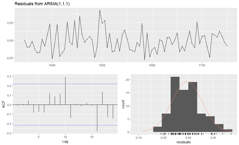
It is important to verify the significance of residuals auto-correlation, in order to see if the spike at lag = 16 is as such. In fact, the purpose of running the LjungBox test is to verify if any auto-correlation beyond the confidence region (as seen in the ACF plot) is a true positive (p-value < 0.05) or is false positive (p-value >= 0.05).
LjungBoxTest(residuals(model_1), k = 2, lag.max = 20)
m    Qm     pvalue
  1  0.01 0.92611002
  2  0.01 0.91139925
  3  0.17 0.68276539
  4  0.82 0.66216496
  5  1.35 0.71745835
  6  1.99 0.73828536
  7  3.32 0.65017878
  8  3.98 0.67886254
  9  5.16 0.64076272
 10 13.34 0.10075806
 11 15.32 0.08260244
 12 15.32 0.12066369
 13 15.35 0.16692082
 14 15.39 0.22084407
 15 15.40 0.28310047
 16 23.69 0.04989871
 17 25.63 0.04204503
 18 27.65 0.03480954
 19 30.06 0.02590249
 20 30.07 0.03680262
The p-value at lag = 16 is < 0.05 hence the auto-correlation spike at lag = 16 out of the confidence interval is significative. Our model #1 has not captured all the structure of the original time series. Also auto-correlations at lags = {17, 18, 19, 20} have p-value < 0.05, however they stand within the confidence inteval.
Now doing the same with sarima() function.
sarima(excess_ts, p = 1, d = 1, q = 1)
Gives this plot.

The sarima() output plot shows results congruent with previous comments.
Model #2 Residuals Diagnostic
Checking ARIMA (1,0,0)(0,0,1)[10] model residuals.
checkresiduals(model_2)
Gives this plot.
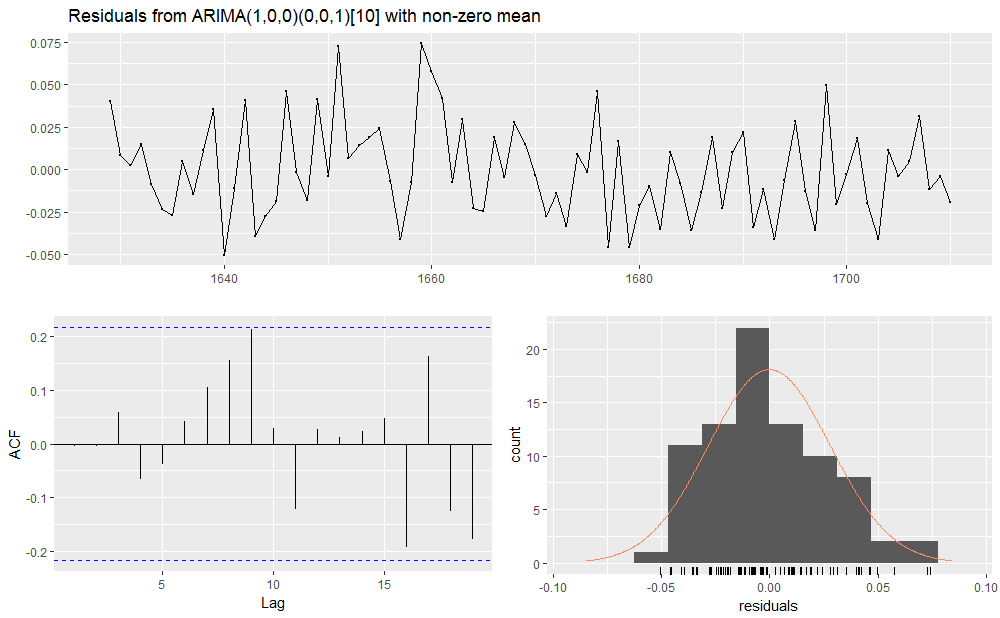
We observe how the model #2 does not show auto-correlation spikes above the confidence interval, and that is a confirmation of the presence of seasonality with period = 10.
LjungBoxTest(residuals(model_2), k = 2, lag.max = 20)
m    Qm    pvalue
  1  0.00 0.9674875
  2  0.00 0.9545816
  3  0.30 0.5815774
  4  0.69 0.7096699
  5  0.82 0.8442508
  6  0.98 0.9121811
  7  2.01 0.8481327
  8  4.24 0.6442302
  9  8.56 0.2861290
 10  8.63 0.3742209
 11 10.06 0.3459882
 12 10.13 0.4290298
 13 10.15 0.5172343
 14 10.20 0.5985932
 15 10.44 0.6577499
 16 14.30 0.4275627
 17 17.14 0.3104476
 18 18.86 0.2759461
 19 22.35 0.1715052
 20 22.41 0.2142307
No p-value > 0.05 are shown by the LjungBox test report. Now showing sarima() plots.
sarima(excess_ts, p = 1, d = 0, q = 0, P = 0, D = 0, Q = 1, S = 10)
Gives this plot.

The sarima() output plot shows results congruent with previous comments. As a conclusion, model #2 has white noise residuals.
Model #3 Residuals Diagnostic
Checking ARIMA (1,0,0)(1,0,0)[10] model residuals.
checkresiduals(model_3)
Gives this plot.
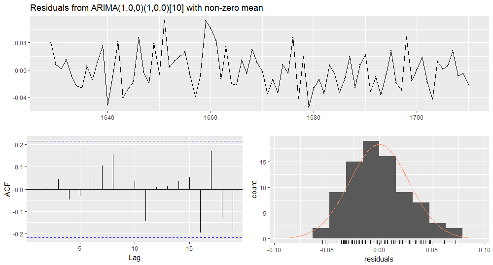
LjungBoxTest(residuals(model_3), k = 2, lag.max = 20)
m    Qm    pvalue
  1  0.00 0.9583318
  2  0.00 0.9553365
  3  0.18 0.6719971
  4  0.37 0.8313599
  5  0.46 0.9285781
  6  0.63 0.9600113
  7  1.63 0.8975737
  8  3.90 0.6901431
  9  8.23 0.3126132
 10  8.34 0.4005182
 11 10.36 0.3222430
 12 10.36 0.4091634
 13 10.39 0.4960029
 14 10.52 0.5708185
 15 10.78 0.6290166
 16 14.81 0.3914043
 17 17.91 0.2675070
 18 19.69 0.2343648
 19 23.37 0.1374412
 20 23.70 0.1651785
sarima(excess_ts, p = 1, d = 0, q = 0, P = 1, D = 0, Q = 0, S = 10)
Gives this plot.
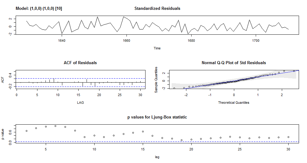
Model#3 has white noise residuals.
Model #4 Residuals Diagnostic
Checking residuals of the ARIMA (0,0,0)(0,0,1)[10] model with level shift.
checkresiduals(model_4)
Gives this plot.
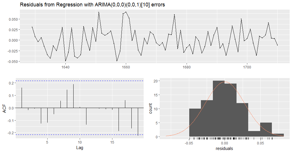
LjungBoxTest(residuals(model_4), k = 1, lag.max = 20)
m    Qm    pvalue
  1  2.20 0.1379312
  2  2.23 0.1349922
  3  2.24 0.3262675
  4  3.68 0.2977682
  5  4.99 0.2884494
  6  5.23 0.3884858
  7  5.52 0.4787801
  8  7.45 0.3837810
  9 10.78 0.2142605
 10 10.79 0.2905934
 11 12.61 0.2465522
 12 12.61 0.3198632
 13 12.61 0.3979718
 14 12.63 0.4769589
 15 12.65 0.5538915
 16 16.37 0.3578806
 17 16.77 0.4005631
 18 19.73 0.2882971
 19 25.25 0.1182396
 20 25.31 0.1504763
sarima(excess_ts, p = 0, d = 0, q = 0, P = 0, D = 0, Q = 1, S = 10, xreg = level)
Gives this plot.
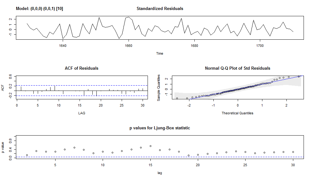
As a conclusion, model #4 has white noise residuals.
Model #6 Residuals Diagnostic
Checking residuals of the ARIMA (1,0,0) model with level shift.
checkresiduals(model_6)
Gives this plot
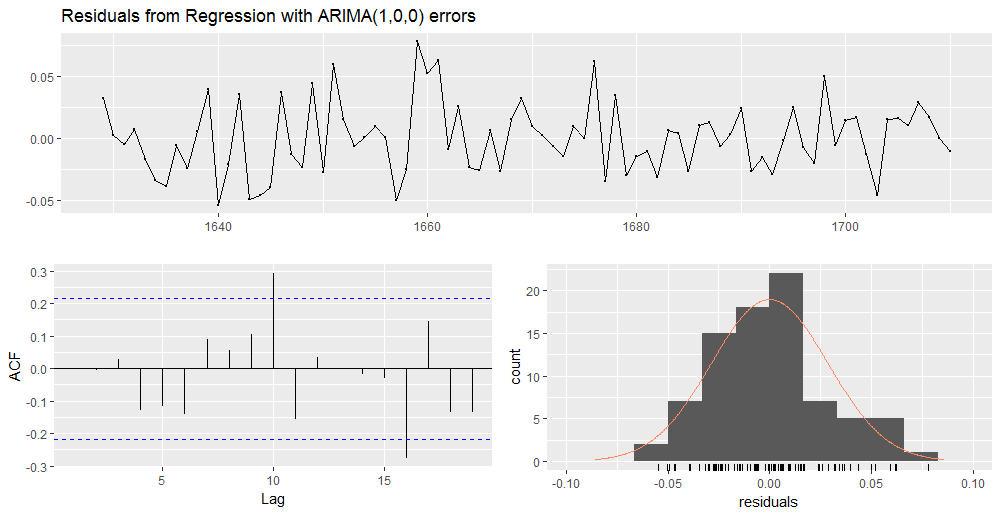
We can observe ACF spikes above the confidence region for lags = {10, 16}.
LjungBoxTest(residuals(model_6), k = 1, lag.max = 20)
m    Qm     pvalue
  1  0.00 0.99713258
  2  0.00 0.96036600
  3  0.07 0.96612792
  4  1.51 0.67947886
  5  2.70 0.60998895
  6  4.47 0.48361437
  7  5.20 0.51895133
  8  5.49 0.59997164
  9  6.51 0.58979614
 10 14.72 0.09890580
 11 17.09 0.07239050
 12 17.21 0.10175761
 13 17.21 0.14179063
 14 17.24 0.18844158
 15 17.34 0.23872998
 16 25.31 0.04596230
 17 27.53 0.03591335
 18 29.50 0.03021450
 19 31.47 0.02537517
 20 31.71 0.03370585
The LjungBox test reports the residuals auto-correlation at lag = 10 as not significative (p-value > 0.05). The lag = 16 residuals auto-correlation is significative (p-value < 0.05). Let us do same verifications with sarima().
sarima(excess_ts, p = 1, d = 0, q = 0, xreg = level)
Gives this plot.
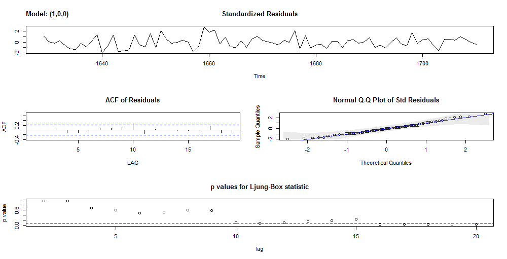
The sarima() plots confirm the presence of significative auto-correlations in the residuals at lag = 16. As a conclusion, this model does not capture all the structure of our original time series.
As overall conclusion, only the seasonal models have white noise residuals.
Models Summary
Finally, it is time to gather the overall AIC, AICc and BIC metrics of our five candidate models (please remember that model #5 has been cut off from the prosecution of the analysis) and choose the final model.
df <- data.frame(col_1_res = c(model_1$aic, model_2$aic, model_3$aic, model_4$aic, model_6$aic),
                    col_2_res = c(model_1$aicc, model_2$aicc, model_3$aicc, model_4$aicc, model_6$aicc),
                    col_3_res = c(model_1$bic, model_2$bic, model_3$bic, model_4$bic, model_6$bic))

colnames(df) <- c("AIC", "AICc", "BIC")
rownames(df) <- c("ARIMA(1,1,1)",
                  "ARIMA(1,0,0)(0,0,1)[10]",
                  "ARIMA(1,0,0)(1,0,0)[10]",
                  "ARIMA(0,0,0)(0,0,1)[10] with level shift",
                  "ARIMA(1,0,0) with level shift")
df
                                               AIC      AICc         BIC
ARIMA(1,1,1)	                           -329.8844	-329.5727   -322.7010
ARIMA(1,0,0)(0,0,1)[10]	                   -344.4575	-343.9380   -334.8306
ARIMA(1,0,0)(1,0,0)[10]	                   -344.1906	-343.6711   -334.5637
ARIMA(0,0,0)(0,0,1)[10] with level shift   -348.8963	-348.3768   -339.2694
ARIMA(1,0,0) with level shift	           -343.3529	-342.8334   -333.7260
The model which provides the best AIC, AICc and BIC metrics at the same time is model #4, ARIMA(0,0,0)(0,0,1)[10] with level shift.
Note: In case of structural changes, the (augmented) Dickey-Fuller test is biased toward the non rejection of the null, as ref. [2] explains. This may justify why the null hypothesis of unit root presence was not rejected by such test and model #1 performs worse than the other ones in terms of AIC metric. Further, you may verify that with d=1 in models from #2 up to #6, the AIC metric does not improve.
Forecast
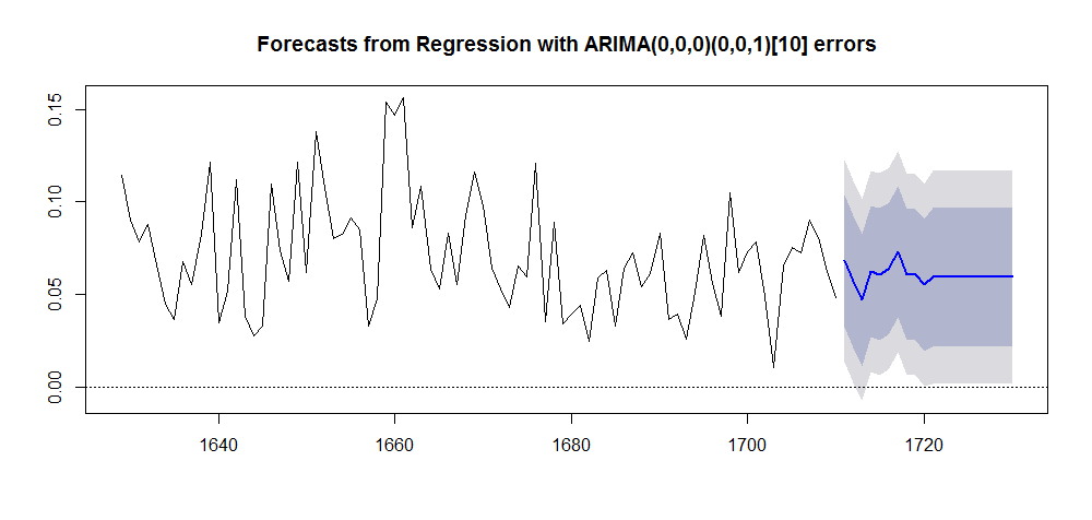
I take advantage of the forecast() function provided within forecast package using model #4 as input. The xreg variable is determined as a constant level equal to one congruently with the structural analysis results.
h_fut <- 20
plot(forecast(model_4, h = h_fut, xreg = rep(1, h_fut)))
Gives this plot.
Historical Background
So we observed a level shift equal approximately to 2.25% in the boys vs girls births excess ratio occurring on year 1670. Two questions arises:
1. What could have influenced the sex-ratio at birth ?
2. What was happening in London during the 17-th century ?
There are studies showing results in support of the fact that sex-ratio at birth is influenced by war periods. Studies such as ref. [7], [8] and [9] suggest an increase of boys births during and/or after war time. General justification is for an adaptive response to external conditions and stresses. Differently, studies as ref. [10] state that there is no statistical evidence of war time influence on sex-ratio at births. Under normal circumstances, the boys vs girls sex ratio at birth is approximately 105:100 on average, (according to some sources), and generally between 102:100 and 108:100.
Our time series covers most of the following eras of the England history (ref. [11]):
* Early Stuart era: 1603-1660
* Later Stuart era 1660-1714
The English Civil War occured during the Early Stuart era and consisted of a series of armed conflicts and political machinations that took place between Parliamentarians (known as Roundheads) and Royalists (known as Cavaliers) between 1642 and 1651. The English conflict left some 34,000 Parliamentarians and 50,000 Royalists dead, while at least 100,000 men and women died from war-related diseases, bringing the total death toll caused by the three civil wars in England to almost 200,000 (see ref. [12]).
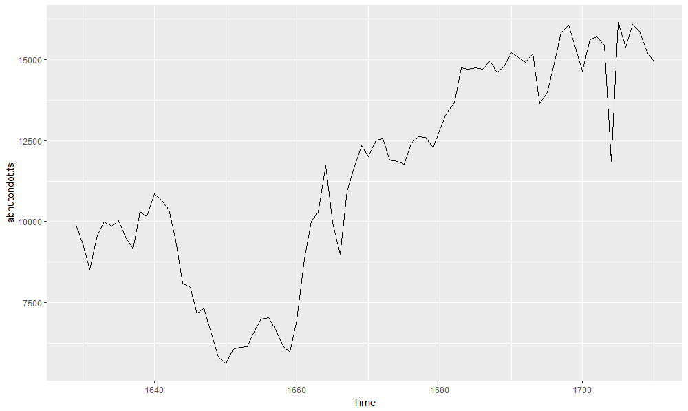
If we step back to view the first plot showing the abhutondot dataset, we can observe a sharp drop on births (both boys and girls) between 1642 and 1651, as testify a period of scarce resources and famine, and we can infer it was due to the civil war. Let us run a quick analysis on the total number of births.
abhutondot.ts <- ts(abhutondot$boys + abhutondot$girls, frequency = 1 ,
                    start = abhutondot$year[1])
autoplot(abhutondot.ts)
Gives this plot.
I then verify if any structural breaks are there with respect a constant level as regressor.
summary(lm(abhutondot.ts ~ 1))
Call:
lm(formula = abhutondot.ts ~ 1)

Residuals:
    Min      1Q  Median      3Q     Max
-5829.7 -2243.0   371.3  3281.3  4703.3

Coefficients:
            Estimate Std. Error t value Pr(>|t|)
(Intercept)    11442        358   31.96   <2e-16 ***
---
Signif. codes:  0 ‘***’ 0.001 ‘**’ 0.01 ‘*’ 0.05 ‘.’ 0.1 ‘ ’ 1

Residual standard error: 3242 on 81 degrees of freedom
The regression is reported as significative. Going on with the search for structural breaks, if any.
(break_point <- breakpoints(abhutondot.ts ~ 1))
	 Optimal 4-segment partition:

Call:
breakpoints.formula(formula = abhutondot.ts ~ 1)

Breakpoints at observation number:
15 33 52

Corresponding to breakdates:
1643 1661 1680
plot(break_point)
Gives this plot.
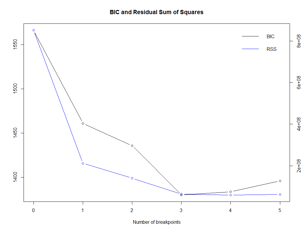
summary(break_point)
	 Optimal (m+1)-segment partition:
Call:
breakpoints.formula(formula = abhutondot.ts ~ 1)

Breakpoints at observation number:

m = 1         39
m = 2      33    52
m = 3   15 33    52
m = 4   15 33    52 68
m = 5   15 32 44 56 68

Corresponding to breakdates:

m = 1             1667
m = 2        1661      1680
m = 3   1643 1661      1680
m = 4   1643 1661      1680 1696
m = 5   1643 1660 1672 1684 1696

Fit:

m   0         1         2         3         4         5
RSS 851165494 211346686 139782582  63564154  59593922  62188019
BIC      1566      1461      1436      1380      1383      1396
The BIC minimum value is reached with m = 3. Let us plot the original time series against its structural breaks and their confidence intervals.
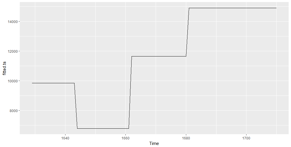
plot(abhutondot.ts)
fitted.ts <- fitted(break_point, breaks = 3)
lines(fitted.ts, col = 4)
lines(confint(break_point, breaks = 3))
Gives this plot.
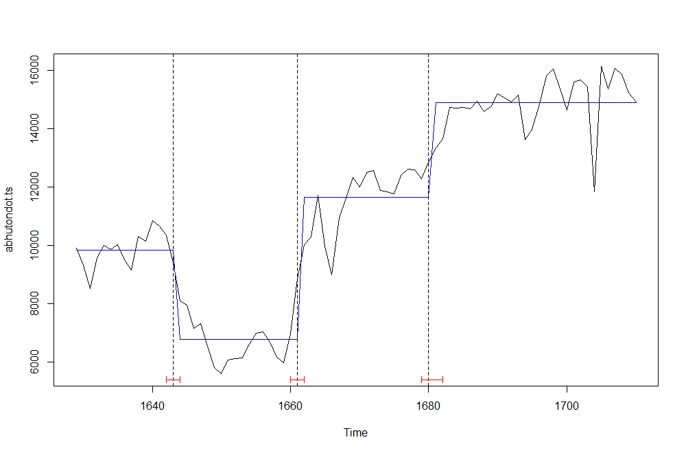
The fitted levels and the breakpoints dates are as follows.
unique(as.integer(fitted.ts))
[1] 9843 6791 11645 14902
breakdates(break_point, breaks = 3)
[1] 1648 1663 1676
So it is confirmed that the total number of births went through a sequence of level shift due to exogeneous shocks. The civil war is very likely determining the first break and its end the second one. It is remarkable the total births decrease from the 9843 level down to 6791 occurring around year 1648. As well remarkable, the level up shift happened on year 1663, afterwards the civil war end. The excess sex ratio structural break on year 1670 occurred at a time approximately in between total births second and third breaks.
The fitted multiple level shifts (as determined by the structural breaks analysis) can be used as intervention variable to fit an ARIMA model, as shown below.
fitted.ts <- fitted(break_point, breaks = 3)
autoplot(fitted.ts)
Gives this plot.
abhutondot_xreg <- Arima(abhutondot.ts, order = c(0,1,1), xreg = fitted.ts, include.mean = TRUE)
summary(abhutondot_xreg)
Series: abhutondot.ts
Regression with ARIMA(0,1,1) errors

Coefficients:
          ma1  fitted.ts
      -0.5481     0.5580
s.e.   0.1507     0.1501

sigma^2 estimated as 743937:  log likelihood=-661.65
AIC=1329.3   AICc=1329.61   BIC=1336.48

Training set error measures:
                   ME     RMSE      MAE       MPE    MAPE     MASE       ACF1
Training set 71.60873 846.5933 622.1021 0.0132448 5.92764 1.002253 0.08043183
coeftest(abhutondot_xreg)
z test of coefficients:

          Estimate Std. Error z value  Pr(>|z|)
ma1       -0.54809    0.15071 -3.6368 0.0002761 ***
fitted.ts  0.55799    0.15011  3.7173 0.0002013 ***
---
Signif. codes:  0 ‘***’ 0.001 ‘**’ 0.01 ‘*’ 0.05 ‘.’ 0.1 ‘ ’ 1
checkresiduals(abhutondot_xreg)
Gives this plot.
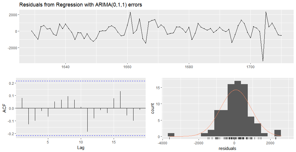
LjungBoxTest(residuals(abhutondot_xreg), k=1, lag.max=20)
m    Qm    pvalue
  1  1.39 0.2387836
  2  2.26 0.1325458
  3  2.31 0.3156867
  4  2.69 0.4416912
  5  2.93 0.5701546
  6  3.32 0.6503402
  7  4.14 0.6580172
  8  4.53 0.7170882
  9  4.54 0.8054321
 10  7.86 0.5479118
 11  8.51 0.5791178
 12  8.54 0.6644773
 13  8.69 0.7292904
 14  9.31 0.7491884
 15 11.16 0.6734453
 16 11.50 0.7163115
 17 12.58 0.7035068
 18 12.60 0.7627357
 19 13.01 0.7906889
 20 14.83 0.7334703
sarima(abhutondot.ts, p=0, d=1, q=1, xreg = fitted.ts)
Gives this plot.
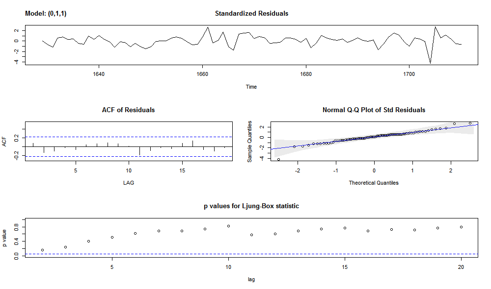
The residuals are white noise.
Conclusions
To have spot seasonality and level shifts were important aspects in our ARIMA models analysis. The seasonal component allowed to define models with white noise residuals. The structural breaks analysis allowed to define models with improved AIC metric introducing as regressor the identified level shifts. We also had the chance to go through some historical remarks of the history of England and get to know about sex ratio at birth studies.
If you have any questions, please feel free to comment below.
References
- [1] Applied Econometrics with R, Achim Zeileis, Christian Kleiber – Springer Ed.
[2] Applied Econometrics Time Series, Walter Enders – Wiley Ed.
[3] Intervention Analysis – Penn State, Eberly College of Science – STAT510
[4] Forecast Package
[5] Seasonal Periods – Rob J. Hyndman
[6] Time Series Analysis With Applications in R – Jonathan D. Cryer, Kung.Sik Chan – Springer Ed.,
[7] Why are more boys born during war ? – Dirk Bethmann, Michael Kvasnicka
[8] Evolutionary ecology of human birth sex ratio – Samuli Helle, Samuli Helama, Kalle Lertola
[9] The Sex Ratio at Birth Following Periods of Conflict – Patrick Clarkin
[10] The ratio of male to female births as affected by wars – E. R. Shaw – American Statistical Association
[11] Early Modern Britain – Wikipedia
[12] English Civil Wars