
In October 2025, 63.1% of US adults said they would cover a surprise $400 expense with cash or its equivalent (money already in the bank, or a credit card paid off at the next statement). That is the Federal Reserve Board’s Survey of Household Economics and Decisionmaking, which asked 12,934 adults. The other 36.9% would borrow, sell something, carry a balance or not pay at all. Renters stand out: 60.1% of them would come up short, against 24.0% of homeowners.
I wanted to know how much of that gap is left once you compare renters and owners with the same income, education, age and family situation, since those differ a lot between the two groups. The standard tool is logistic regression, and its standard output, the odds ratio, is where the answer goes wrong. On this data the adjusted odds ratio for renting is 1.93, which gets read as "renters are almost twice as likely to be short of $400". From the same fitted model, the risk ratio is 1.36: at the same income, education, age, race and household, renters are 36% more likely to come up short, not 93%.
How do I get a risk ratio from a logistic regression in R?
Average the model’s predicted probabilities twice, once with everyone set to the reference group and once with everyone set to the comparison group, then divide. avg_comparisons() from marginaleffects does this with comparison = "ratio" and adds a confidence interval. This block runs on its own (R 4.6.1, survey 4.5, marginaleffects 1.0.0): it downloads the Fed’s public-use file, a 4.5 MB zip that needs no key, fits a survey-weighted logistic regression and prints both numbers.
library(tidyverse)
library(survey)
library(marginaleffects)

zip <- tempfile(fileext = ".zip")
download.file("https://www.federalreserve.gov/consumerscommunities/files/SHED_public_use_data_2025_(CSV).zip",
              zip, mode = "wb")

shed <- read_csv(unz(zip, "public2025.csv"), show_col_types = FALSE,
                 col_select = c(weight, pay_casheqv, GH1, ppinc7, ppeducat,
                                ppethm, ppagecat, ppmarit5, ppkid017)) |>
  mutate(short   = pay_casheqv == "No",   # would not cover $400 with cash or equivalent
         tenure  = case_when(GH1 == "Pay rent" ~ "Rent",
                             GH1 == "Neither own nor pay rent" ~ "Neither",
                             .default = "Own") |> factor(c("Own", "Rent", "Neither")),
         income  = fct_relevel(ppinc7, "$150,000 or more"),
         educ    = fct_relevel(ppeducat, "Bachelor's degree or higher"),
         race    = fct_relevel(ppethm, "White, Non-Hispanic"),
         age     = fct_relevel(ppagecat, "65-74"),
         married = ppmarit5 == "Now married",
         kids    = ppkid017 > 0)

des <- svydesign(ids = ~1, weights = ~weight, data = shed)
fit <- svyglm(short ~ tenure + income + educ + age + race + married + kids,
              design = des, family = quasibinomial())

exp(coef(fit))["tenureRent"]    # odds ratio
## tenureRent
##   1.932933
avg_comparisons(fit, variables = list(tenure = c("Own", "Rent")),
                comparison = "ratio", wts = TRUE, hypothesis = 1)    # risk ratio
##
##  Estimate Std. Error    z Pr(>|z|)    S 2.5 % 97.5 %
##      1.36     0.0383 9.41   <0.001 67.5  1.29   1.43
##
## Term: tenure
## Type: response
## Comparison: mean(Rent) / mean(Own)
The odds ratio’s 95% interval runs from 1.72 to 2.17, the risk ratio’s from 1.29 to 1.43. Two arguments in that call are easy to leave out. wts = TRUE makes the averaging use the survey weights; the default, wts = FALSE, averages over respondents as if each counted the same. And hypothesis = 1 tests the ratio against 1, no difference; without it the printed p-value tests whether the ratio is zero, which is never the question. pay_casheqv is the Fed’s own derived variable, so the outcome matches its published 63% figure. The public file has weights but no strata or clusters, so ids = ~1 is as much survey design as it allows.
What avg_comparisons() did is short enough to write out:
p_if <- \(group) {
  everyone <- mutate(shed, tenure = factor(group, levels = levels(tenure)))
  weighted.mean(as.numeric(predict(fit, everyone, type = "response")), shed$weight)
}
c(own = p_if("Own"), rent = p_if("Rent"), ratio = p_if("Rent") / p_if("Own"))
##       own      rent     ratio
## 0.3234843 0.4399367 1.3599942
If every adult in the sample owned their home, the model predicts 32.3% would be short of $400; if every adult rented, 44.0%. The ratio of those two is the risk ratio.
Why the odds ratio runs ahead of the risk
Odds are p / (1 − p), and they stretch as p grows. A 24.0% risk is odds of 0.315; a 60.1% risk is odds of 1.504, 4.77 times as high. The two ratios are tied together by the risk in each group, p0 for the reference group and p1 for the comparison:
$$\text{OR} = \text{RR} \times \frac{1 – p_0}{1 – p_1}$$
On the raw shares, renters’ risk ratio is 2.51 and their odds ratio 2.51 × 0.76 / 0.40 = 4.77. When the outcome is rare, both 1 − p terms are close to 1 and the two ratios agree; the usual rule of thumb is an outcome under 10%. Here 36.9% of adults are short, so they do not. The odds ratio is also the same in both directions, which the risk ratio is not: renters are 2.51 times as likely as owners to be short of $400, and owners are 1.90 times as likely as renters to cover it, while the odds ratio is 4.77 (or its inverse) either way. "Times as likely" is a statement about probabilities, so it needs the risk ratio.
What still matters at the same income
The same gap opens for every characteristic in the model, and it widens as the effect grows. Holding the rest fixed, a household earning $10,000 to $24,999 is 2.51 times as likely as one earning $150,000 or more to be short of $400, where the odds ratio says 6.69. Adults without a high-school diploma are 1.76 times as likely as college graduates (odds ratio 3.33), and Black adults 1.48 times as likely as white adults with the same income, education, age and housing (odds ratio 2.43).
risk <- c("tenure", "income", "educ", "age", "race", "kids") |>
  map(\(v) avg_comparisons(fit, variables = v, comparison = "ratio", wts = TRUE)) |>
  map(as_tibble) |>
  list_rbind() |>
  mutate(coef = paste0(term, str_match(contrast, "^mean\\((.*)\\) / mean")[, 2]))

ratios <- tibble(coef = names(coef(fit)), or = exp(coef(fit))) |>
  inner_join(select(risk, coef, rr = estimate), by = "coef")
dsp_colors <- c("#0066CC", "#E8862D", "#159A6C", "#7D5BD6",
                "#D64580", "#2AA9B8", "#C9A227")
dsp_theme <- theme_minimal(base_size = 13) +
  theme(plot.background    = element_rect(fill = "#ECECEF", color = NA),
        panel.background   = element_rect(fill = "#ECECEF", color = NA),
        panel.grid.minor   = element_blank(),
        panel.grid.major.x = element_blank(),
        panel.grid.major.y = element_line(color = "grey78"),
        axis.ticks         = element_blank(),
        plot.title         = element_text(face = "bold"),
        strip.text         = element_text(face = "bold"))

shown <- c("income$10,000 to $24,999"             = "Income $10-25K vs $150K+",
           "income$25,000 to $49,999"             = "Income $25-50K vs $150K+",
           "income$50,000 to $74,999"             = "Income $50-75K vs $150K+",
           "educNo high school diploma or GED"    = "No high-school diploma vs bachelor's",
           "educHigh school graduate (high school diploma or the equivalent GED)" =
                                                    "High-school graduate vs bachelor's",
           "raceBlack, Non-Hispanic"              = "Black vs white",
           "raceHispanic"                         = "Hispanic vs white",
           "age35-44"                             = "Age 35-44 vs 65-74",
           "tenureRent"                           = "Renting vs owning",
           "kidsTRUE"                             = "Children at home vs none")

ratios |>
  filter(coef %in% names(shown)) |>
  mutate(label = fct_reorder(shown[coef], or)) |>
  pivot_longer(c(rr, or), names_to = "measure", values_to = "ratio") |>
  mutate(measure = factor(measure, c("rr", "or"), c("Risk ratio", "Odds ratio"))) |>
  ggplot(aes(ratio, label)) +
  geom_vline(xintercept = 1, linetype = "dashed", color = "grey40") +
  geom_line(aes(group = label), color = "grey55", linewidth = 1) +
  geom_point(aes(color = measure), size = 3.2) +
  scale_x_log10(breaks = c(1, 1.5, 2, 3, 5, 7), labels = c("1", "1.5", "2", "3", "5", "7")) +
  scale_color_manual(values = dsp_colors) +
  labs(x = "Ratio, same fitted model (log scale)", y = NULL, color = NULL,
       title = "The odds ratio overstates every gap",
       subtitle = "Short of $400 in cash or equivalent, US adults, October 2025") +
  dsp_theme +
  theme(legend.position = "top")
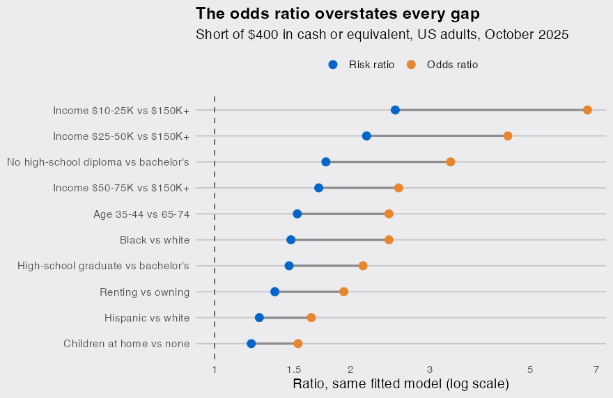
So, on the scale people actually read: in the Fed’s 2025 survey, 37% of US adults could not cover a $400 emergency with cash or its equivalent. Income is by far the strongest predictor. At the same income, education, age, race and household, renting still goes with a 36% higher chance of coming up short, Black adults are 48% more likely than white adults to be short, and adults with children at home are 21% more likely than those without. These are associations in one cross-section, not effects of moving house. On the odds scale, every one of those excesses looks at least 2.2 times as big. When the outcome is common, report the risk ratio from avg_comparisons() next to exp(coef()), or instead of it.
Data: Board of Governors of the Federal Reserve System, Survey of Household Economics and Decisionmaking [dataset] (Washington: Board of Governors, 2026), https://doi.org/10.17016/datasets.002.
