In the second part (first part is here) of this tutorial, we are going to build two types of classification models and compare their performances in terms of accuracy.
Packages
The overall list of packages used for this tutorial (part #1 and part #2) are as follows.
suppressPackageStartupMessages(library(caret))
suppressPackageStartupMessages(library(ggplot2))
suppressPackageStartupMessages(library(dplyr))
suppressPackageStartupMessages(library(gridExtra))
suppressPackageStartupMessages(library(Kmisc))
suppressPackageStartupMessages(library(gmodels))
suppressPackageStartupMessages(library(ggparallel))
suppressPackageStartupMessages(library(rpart.plot))
suppressPackageStartupMessages(library(sqldf))
Classification Models
We are going to take advantage of the caret package (ref. [8]) to build models using rpart and C5.0Rules classification models. As a first step, we define the training and validation datasets and the model formula. The original dataset is split into 60% and 40% proportions to obtain the training dataset and validation datasets. The training procedure will take advantage of cross-validation in number of 10 folds.
url_file <-  "https://archive.ics.uci.edu/ml/machine-learning-databases/mushroom/agaricus-lepiota.data"
mushrooms <- read.csv(url(url_file), header=FALSE)
fields <- c("class",
            "cap_shape",
            "cap_surface",
            "cap_color",
            "bruises",
            "odor",
            "gill_attachment",
            "gill_spacing",
            "gill_size",
            "gill_color",
            "stalk_shape",
            "stalk_root",
            "stalk_surface_above_ring",
            "stalk_surface_below_ring",
            "stalk_color_above_ring",
            "stalk_color_below_ring",
            "veil_type",
            "veil_color",
            "ring_number",
            "ring_type",
            "spore_print_color",
            "population",
            "habitat")

colnames(mushrooms) <- fields

set.seed(1023)
train_idx <- createDataPartition(mushrooms$class, p=0.6, list=FALSE)
trControl <- trainControl(method = "repeatedcv",  number=10, repeats=5, verboseIter=TRUE)

feat_sum <- paste(relevant_features, collapse = "+")
frm <- as.formula(paste("class ~ ", feat_sum))
frm

class ~ cap_shape + cap_surface + cap_color + bruises + odor +
    gill_attachment + gill_spacing + gill_size + gill_color +
    stalk_shape + stalk_root + stalk_surface_above_ring + stalk_surface_below_ring +
    stalk_color_above_ring + stalk_color_below_ring + veil_color +
    ring_number + ring_type + spore_print_color + population +
    habitat
The formula above shall be used in the model we are going to build.
RPART
We are going to take advantage of rpart classification model (ref. [9]) capable to build Recursive Partitioning Tree models. The rpart routine builds classification or regression models of a very general structure using a two stage procedure; the resulting models can be represented as binary trees. The tree is built by the following process: first the single variable is found which best splits the data into two groups (‘best’ according to some criteria). The data is separated, and then this process is applied separately to each sub-group, and so on recursively until the subgroups either reach a minimum size or until no improvement can be made. For further details please see ref. [9].
In the following, we set the threshold complexity parameter, cp, to zero in order to have no costs for adding a split into the output classification tree being build. That has to be done carefully as a low cp value may result in overfitting. The accuracy is the metric we want to take into account.
rpart.grid <- expand.grid(.cp=0)
rpart_fit <- train(frm,
                   data = mushrooms[train_idx,],
                   method ="rpart",
                   trControl = trControl,
                   tuneGrid=rpart.grid,
                   metric = 'Accuracy')
rpart_fit
CART

4875 samples
  21 predictor
   2 classes: 'e', 'p'

No pre-processing
Resampling: Cross-Validated (10 fold)
Summary of sample sizes: 4387, 4387, 4388, 4388, 4387, 4387, ...
Resampling results:

  Accuracy   Kappa
  0.9975385  0.9950708

Tuning parameter 'cp' was held constant at a value of 0
Variables importance report is shown herein below.
varImp(rpart_fit)
rpart variable importance

  only 20 most important variables shown (out of 95)

                          Overall
odorn                     100.000
odorf                      63.133
stalk_surface_above_ringk  60.013
stalk_surface_below_ringk  53.376
gill_sizen                 48.751
bruisest                   38.092
odorl                      37.967
stalk_rootc                29.069
ring_typep                 28.692
habitatm                   18.715
stalk_surface_below_ringy  16.513
stalk_rootr                14.035
spore_print_colorr          4.717
spore_print_coloru          4.123
gill_spacingw               4.047
odorm                       2.987
stalk_surface_above_rings   2.987
stalk_surface_below_rings   2.987
stalk_color_below_ringy     2.019
cap_colory                  1.892
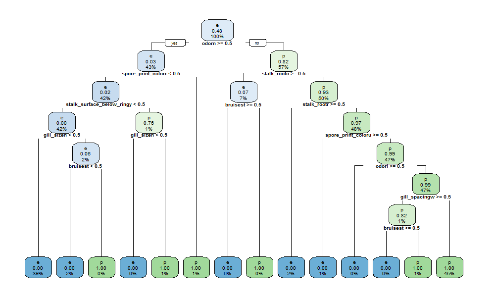
To have no odor or a foul odor are considered relevant details in determining if mushrooms are edible or poisonous. To evaluate stalk surface and gill size are further aspects to be considered. We then verify our model against the validation dataset.
rpart_test_pred <- predict(rpart_fit, mushrooms[-train_idx,])
confusionMatrix(rpart_test_pred, mushrooms[-train_idx,]$class)
Confusion Matrix and Statistics

          Reference
Prediction    e    p
         e 1683    0
         p    0 1566

               Accuracy : 1
                 95% CI : (0.9989, 1)
    No Information Rate : 0.518
    P-Value [Acc > NIR] : < 2.2e-16

                  Kappa : 1
 Mcnemar's Test P-Value : NA

            Sensitivity : 1.000
            Specificity : 1.000
         Pos Pred Value : 1.000
         Neg Pred Value : 1.000
             Prevalence : 0.518
         Detection Rate : 0.518
   Detection Prevalence : 0.518
      Balanced Accuracy : 1.000

       'Positive' Class : e
100% accuracy is achieved. Plot of the resulting classification model is shown.
rpart.plot(rpart_fit$finalModel, cex=0.6)
C5.0Rules
Decision trees can sometimes be quite difficult to understand. An important feature of C5.0 is its ability to generate classifiers called rulesets that consist of unordered collections of (relatively) simple if-then rules (ref. [10] and [11]). We are going to take advantage of the same train control directive and target metric.
c50_fit <- train(frm,
                  data = mushrooms[train_idx,],
                  method ="C5.0Rules",
                  trControl = trControl,
                  metric = 'Accuracy')
c50_fit
Single C5.0 Ruleset

4875 samples
  21 predictor
   2 classes: 'e', 'p'

No pre-processing
Resampling: Cross-Validated (10 fold)
Summary of sample sizes: 4388, 4388, 4388, 4387, 4387, 4387, ...
Resampling results:

  Accuracy  Kappa
  1         1
Variables importance is shown.
varImp(c50_fit)

C5.0Rules variable importance

  only 20 most important variables shown (out of 95)

                          Overall
odorn                      100.00
bruisest                    72.92
stalk_rootc                 57.34
stalk_rootr                 52.84
gill_spacingw               51.58
spore_print_colorr          44.79
gill_sizen                  44.69
stalk_surface_below_ringy   20.38
cap_shapex                   0.00
veil_colory                  0.00
populationy                  0.00
ring_typen                   0.00
gill_coloro                  0.00
cap_colorc                   0.00
spore_print_coloru           0.00
habitatu                     0.00
stalk_color_below_ringc      0.00
spore_print_colork           0.00
cap_surfaces                 0.00
habitatw                     0.00
As for rpart model, to have no odor is the most important feature. Bruise and stalk characteristics follow. In case of C5.0Rules, the important variables are less than rpart ones. So, C5.0Rules model was capable to focus on a smaller variable set to achieve the same accuracy as we will evaluate later also for the validation dataset.
summary(c50_fit)

Rules:

Rule 1: (1926, lift 1.9)
	odorn > 0
	gill_sizen <= 0
	spore_print_colorr   class e  [0.999]

Rule 2: (867, lift 1.9)
	bruisest  0
	stalk_surface_below_ringy   class e  [0.999]

Rule 3: (313, lift 1.9)
	bruisest > 0
	stalk_rootc > 0
	->  class e  [0.997]

Rule 4: (116, lift 1.9)
	stalk_rootr > 0
	->  class e  [0.992]

Rule 5: (61, lift 1.9)
	bruisest > 0
	odorn  0
	->  class e  [0.984]

Rule 6: (2200, lift 2.1)
	odorn <= 0
	gill_spacingw <= 0
	stalk_rootc <= 0
	stalk_rootr   class p  [1.000]

Rule 7: (1948, lift 2.1)
	bruisest <= 0
	odorn   class p  [0.999]

Rule 8: (37, lift 2.0)
	spore_print_colorr > 0
	->  class p  [0.974]

Rule 9: (26, lift 2.0)
	gill_sizen > 0
	stalk_surface_below_ringy > 0
	->  class p  [0.964]

Rule 10: (7, lift 1.8)
	bruisest > 0
	odorn > 0
	gill_sizen > 0
	->  class p  [0.889]

Default class: e


Evaluation on training data (4875 cases):

	        Rules
	  ----------------
	    No      Errors

	    10    0( 0.0%)   <<


	   (a)   (b)    <-classified as
	  ----  ----
	  2525          (a): class e
	        2350    (b): class p


	Attribute usage:

	 89.91%	odorn
	 65.56%	bruisest
	 51.55%	stalk_rootc
	 47.51%	stalk_rootr
	 46.38%	gill_spacingw
	 40.27%	spore_print_colorr
	 40.18%	gill_sizen
	 18.32%	stalk_surface_below_ringy
Each rule consists of:
* a rule number — this is quite arbitrary and serves only to identify the rule.
* statistics (n, lift x) or (n/m, lift x) that summarize the performance of the rule. Similarly to a leaf, n is the number of training cases covered by the rule and m, if it appears, shows how many of them do not belong to the class predicted by the rule. The rule’s accuracy is estimated by the Laplace ratio (n-m+1)/(n+2). The lift x is the result of dividing the rule’s estimated accuracy by the relative frequency of the predicted class in the training set.
* one or more conditions that must all be satisfied if the rule is to be applicable.
* a class predicted by the rule
* a value between 0 and 1 that indicates the confidence with which this prediction is made
Now we will evaluate our model against the validation set.
c50_test_pred <- predict(c50_fit, mushrooms[-train_idx,])
confusionMatrix(c50_test_pred, mushrooms[-train_idx,]$class)
Confusion Matrix and Statistics

          Reference
Prediction    e    p
         e 1683    0
         p    0 1566

               Accuracy : 1
                 95% CI : (0.9989, 1)
    No Information Rate : 0.518
    P-Value [Acc > NIR] : < 2.2e-16

                  Kappa : 1
 Mcnemar's Test P-Value : NA

            Sensitivity : 1.000
            Specificity : 1.000
         Pos Pred Value : 1.000
         Neg Pred Value : 1.000
             Prevalence : 0.518
         Detection Rate : 0.518
   Detection Prevalence : 0.518
      Balanced Accuracy : 1.000

       'Positive' Class : e
100% accuracy reached by C5.0Rules as well.
Comparing Models
The caret package allows for comparing models performances. The resamples function can be used to collect, summarize and contrast the resampling results. Since the random number seeds were initialized to the same value prior to calling train, the same folds were used for each model (ref. [12]).
results <- resamples(list(RPART=rpart_fit, C5.0Rules=c50_fit))
bwplot(results)
Gives this plot:
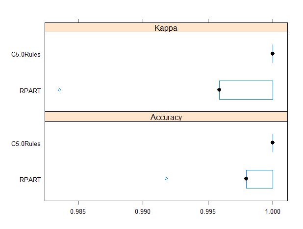
It results C5.0Rules model is slightly more reliable than rpart based one as it provides a higher minimum accuracy.
Further Considerations
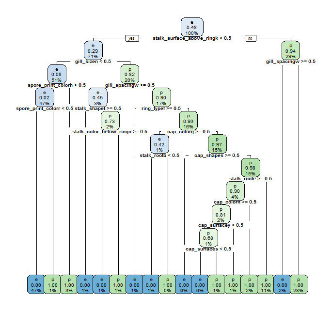
What if only features related to visual characteristics of mushrooms were available? We are going to recompute our models with a subset of the features available, only those immediately visually observable. At the purpose we define a new set of features and corresponding model formula.
relevant_features_2 <- setdiff(relevant_features,
                               c("population", "habitat", "odor", "bruises"))
feat_sum <- paste(relevant_features_2, collapse = "+")
frm <- as.formula(paste("class ~ ", feat_sum))
frm

class ~ cap_shape + cap_surface + cap_color + gill_attachment +
    gill_spacing + gill_size + gill_color + stalk_shape + stalk_root +
    stalk_surface_above_ring + stalk_surface_below_ring + stalk_color_above_ring +
    stalk_color_below_ring + veil_color + ring_number + ring_type +
    spore_print_color
With rpart:
rpart.grid <- expand.grid(.cp=0)
rpart_fit <- train(frm,
                   data = mushrooms[train_idx,],
                   method ="rpart",
                   trControl = trControl,
                   tuneGrid=rpart.grid,
                   metric = 'Accuracy')
rpart_fit
CART

4875 samples
  17 predictor
   2 classes: 'e', 'p'

No pre-processing
Resampling: Cross-Validated (10 fold)
Summary of sample sizes: 4388, 4388, 4387, 4388, 4387, 4387, ...
Resampling results:

  Accuracy   Kappa
  0.9991803  0.9983589

Tuning parameter 'cp' was held constant at a value of 0
varImp(rpart_fit)
rpart variable importance

  only 20 most important variables shown (out of 75)

                          Overall
gill_sizen                100.000
stalk_surface_below_ringk  66.448
ring_typep                 61.468
stalk_surface_above_ringk  57.196
stalk_surface_above_rings  38.960
spore_print_colorh         35.409
spore_print_colorw         25.831
gill_spacingw              14.703
cap_surfaces               13.711
ring_numbert               11.714
ring_numbero                9.179
spore_print_colorr          9.136
cap_colorw                  6.227
ring_typef                  5.981
stalk_shapet                5.937
spore_print_coloru          4.092
stalk_rootb                 3.868
cap_colorg                  3.504
stalk_roote                 3.451
stalk_color_below_ringn     2.548
rpart_test_pred <- predict(rpart_fit, mushrooms[-train_idx,])
confusionMatrix(rpart_test_pred, mushrooms[-train_idx,]$class)

Confusion Matrix and Statistics

          Reference
Prediction    e    p
         e 1683    0
         p    0 1566

               Accuracy : 1
                 95% CI : (0.9989, 1)
    No Information Rate : 0.518
    P-Value [Acc > NIR] : < 2.2e-16

                  Kappa : 1
 Mcnemar's Test P-Value : NA

            Sensitivity : 1.000
            Specificity : 1.000
         Pos Pred Value : 1.000
         Neg Pred Value : 1.000
             Prevalence : 0.518
         Detection Rate : 0.518
   Detection Prevalence : 0.518
      Balanced Accuracy : 1.000

       'Positive' Class : e
rpart.plot(rpart_fit$finalModel, cex=0.6)
Gives this plot:
Now with C5.0Rules.
c50_fit <- train(frm,
                  data = mushrooms[train_idx,],
                  method ="C5.0Rules",
                  trControl = trControl,
                  metric = 'Accuracy')
c50_fit
Single C5.0 Ruleset

4875 samples
  17 predictor
   2 classes: 'e', 'p'

No pre-processing
Resampling: Cross-Validated (10 fold)
Summary of sample sizes: 4388, 4387, 4388, 4387, 4388, 4388, ...
Resampling results:

  Accuracy  Kappa
  1         1
varImp(c50_fit)

C5.0Rules variable importance

  only 20 most important variables shown (out of 75)

                          Overall
gill_sizen                 100.00
stalk_surface_above_ringk   83.17
spore_print_colorh          70.47
spore_print_colorr          49.81
spore_print_colorw          44.94
gill_spacingw               31.60
stalk_rootb                 27.40
stalk_color_below_ringn     26.02
stalk_shapet                23.25
cap_surfacey                21.25
ring_typef                  14.68
cap_surfaces                10.13
gill_colorh                  0.00
ring_numbert                 0.00
cap_shapek                   0.00
gill_colory                  0.00
stalk_color_below_ringw      0.00
gill_colorr                  0.00
veil_coloro                  0.00
ring_typen                   0.00
summary(c50_fit)
Call:
Rules:

Rule 1: (2267, lift 1.9)
	gill_sizen <= 0
	stalk_surface_above_ringk <= 0
	spore_print_colorh <= 0
	spore_print_colorr   class e  [1.000]

Rule 2: (328, lift 1.9)
	cap_surfaces <= 0
	cap_surfacey <= 0
	stalk_rootb <= 0
	stalk_surface_above_ringk   class e  [0.997]

Rule 3: (88, lift 1.9)
	gill_spacingw > 0
	stalk_surface_above_ringk > 0
	->  class e  [0.989]

Rule 4: (61, lift 1.9)
	gill_sizen > 0
	stalk_shapet > 0
	spore_print_colorw   class e  [0.984]

Rule 5: (34, lift 1.9)
	stalk_surface_above_ringk  0
	->  class e  [0.972]

Rule 6: (29, lift 1.9)
	ring_typef > 0
	->  class e  [0.968]

Rule 7: (919, lift 2.1)
	stalk_shapet  0
	spore_print_colorw   class p  [0.999]

Rule 8: (940, lift 2.1)
	gill_sizen  0
	->  class p  [0.999]

Rule 9: (1065, lift 2.1)
	gill_sizen > 0
	stalk_color_below_ringn  0
	->  class p  [0.999]

Rule 10: (1350, lift 2.1)
	gill_spacingw  0
	->  class p  [0.999]

Rule 11: (639, lift 2.1)
	cap_surfacey > 0
	gill_sizen > 0
	stalk_color_below_ringn <= 0
	ring_typef   class p  [0.998]

Rule 12: (133, lift 2.1)
	cap_surfaces > 0
	gill_sizen > 0
	stalk_shapet   class p  [0.993]

Default class: e


Evaluation on training data (4875 cases):

	        Rules
	  ----------------
	    No      Errors

	    12    0( 0.0%)   <<


	   (a)   (b)    <-classified as
	  ----  ----
	  2525          (a): class e
	        2350    (b): class p


	Attribute usage:

	 93.35%	gill_sizen
	 77.64%	stalk_surface_above_ringk
	 65.78%	spore_print_colorh
	 46.50%	spore_print_colorr
	 41.95%	spore_print_colorw
	 29.50%	gill_spacingw
	 25.58%	stalk_rootb
	 24.29%	stalk_color_below_ringn
	 21.70%	stalk_shapet
	 19.84%	cap_surfacey
	 13.70%	ring_typef
	  9.46%	cap_surfaces
c50_test_pred <- predict(c50_fit, mushrooms[-train_idx,])
confusionMatrix(c50_test_pred, mushrooms[-train_idx,]$class)
Confusion Matrix and Statistics

          Reference
Prediction    e    p
         e 1683    0
         p    0 1566

               Accuracy : 1
                 95% CI : (0.9989, 1)
    No Information Rate : 0.518
    P-Value [Acc > NIR] : < 2.2e-16

                  Kappa : 1
 Mcnemar's Test P-Value : NA

            Sensitivity : 1.000
            Specificity : 1.000
         Pos Pred Value : 1.000
         Neg Pred Value : 1.000
             Prevalence : 0.518
         Detection Rate : 0.518
   Detection Prevalence : 0.518
      Balanced Accuracy : 1.000

       'Positive' Class : e
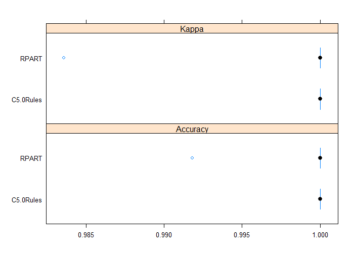
Both rpart and C5.0Rules have been able to achieve 100% accuracy again with a limited increase of complexity for the resulting models compared with the ones using former features set. Let us compare again resulting rpart and C5.0Rules models.
results <- resamples(list(RPART=rpart_fit, C5.0Rules=c50_fit))
bwplot(results)
Gives this plot:
Conclusions
Both rpart and C5.0Rules were able to achieve very high accuracy. We compared them using two features sets. If you have any questions, please feel free to comment below.
References
[1] UCI Machine Learning Archive – Mushroom Dataset
[2] Wikipedia – Mushroom Tutorial
[3] Mushroom Anatomy
[4] Identify Mushrooms
[5] Wikipedia – Universal Veil
[6] Wikipedia – Partial Veil
[7] Mushroom Glossary
[8] Caret package site
[9] rpart package vignette
[10] C5.0 package vignette
[11] C5.0: An Informal Tutorial
[12] Caret Package Vignette
[13] How Decision Tree Algorithms Works