Motivation
In order to predict the Bay area’s home prices, I chose the housing price dataset that was sourced from Bay Area Home Sales Database and Zillow. This dataset was based on the homes sold between January 2013 and December 2015. It has many characteristics of learning, and the dataset can be downloaded from here.
Data Preprocessing
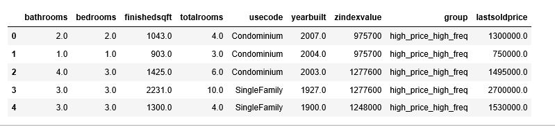
import pandas as pd
sf = pd.read_csv('final_data.csv')
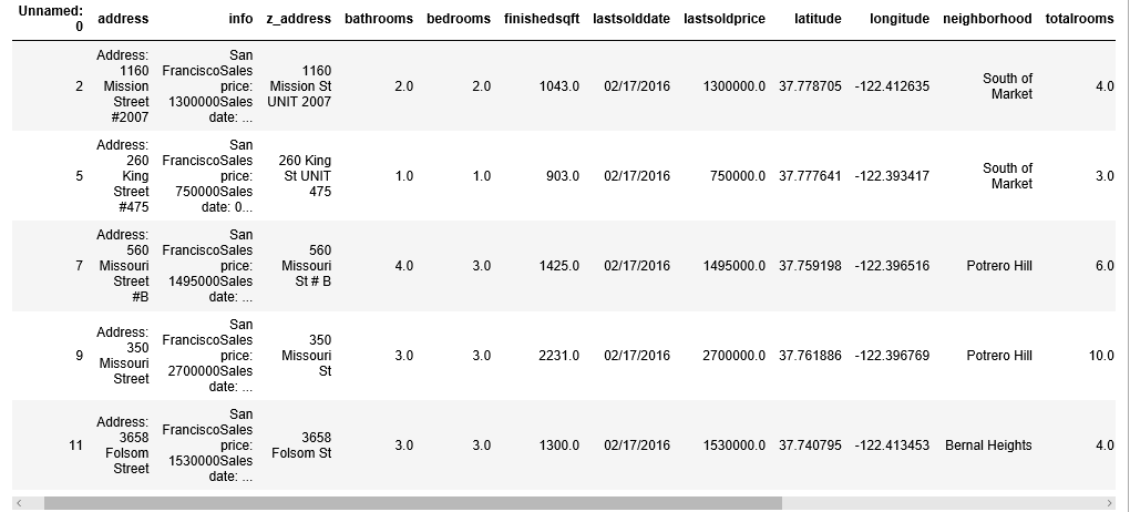
sf.head()
Gives this table:
There are several features that we do not need, such as “info”, “z_address”, “zipcode”(We keep “neighborhood” as a location variable), “zipid” and “zestimate”(This is the price estimated by Zillow, we don’t want our model to be affected by this), so, we will drop them.
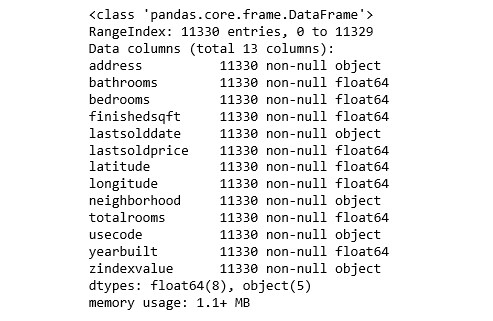
sf.drop(sf.columns[[0, 2, 3, 15, 17, 18]], axis=1, inplace=True)
sf.info()
Gives this table:
The data type of “zindexvalue” should be numeric, so let’s change that.
sf['zindexvalue'] = sf['zindexvalue'].str.replace(',', '')
sf['zindexvalue'] = sf['zindexvalue'].convert_objects(convert_numeric=True)

sf.lastsolddate.min(), sf.lastsolddate.max()
('01/02/2013', '12/31/2015')
The house sold period in the dateset was between January 2013 and December 2015.
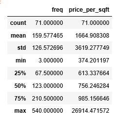
I now use the describe() method to show the summary statistics of the numeric variables.
sf.describe()
Gives this table:
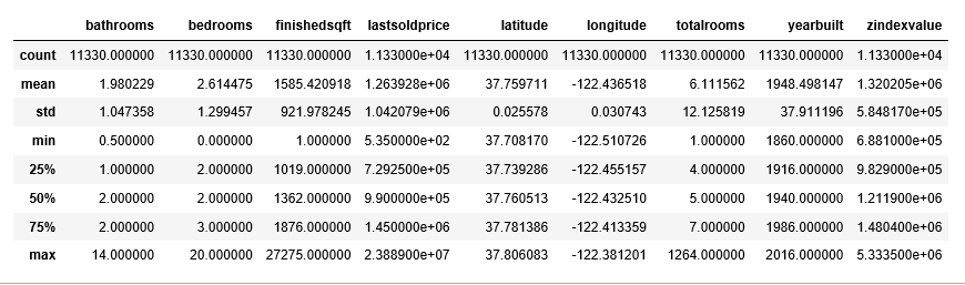
The count, mean, min and max rows are self-explanatory. The std shows the standard deviation, and the 25%, 50% and 75% rows show the corresponding percentiles.
To get a feel for the type of data we are dealing with, we plot a histogram for each numeric variable.
%matplotlib inline
import matplotlib.pyplot as plt
sf.hist(bins=50, figsize=(20,15))
plt.savefig("attribute_histogram_plots")
plt.show()
Gives this plot:
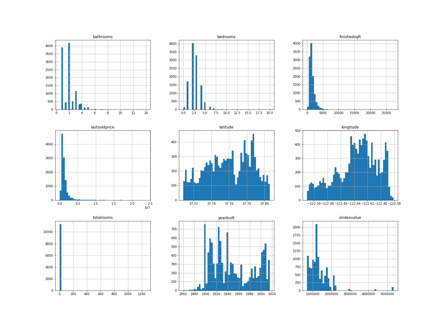
Some of the histograms are a little bit right skewed, but this is not abnormal.
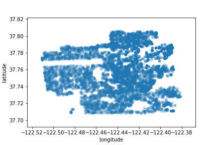
Let’s create a scatter plot with latitude and longitude to visualize the data:
sf.plot(kind="scatter", x="longitude", y="latitude", alpha=0.2)
plt.savefig('map1.png')
Gives this plot:
Now let’s color code from the most expensive to the least expensive areas:
sf.plot(kind="scatter", x="longitude", y="latitude", alpha=0.4, figsize=(10,7), c="lastsoldprice", cmap=plt.get_cmap("jet"), colorbar=True, sharex=False)
plt.savefig('map2.png')
Gives this plot:
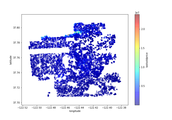
This image tells us that the most expensive houses sold were in the north area.
The variable we are going to predict is the “last sold price”. So let’s look at how much each independent variable correlates with this dependent variable.
corr_matrix = sf.corr()
corr_matrix["lastsoldprice"].sort_values(ascending=False)
lastsoldprice    1.000000
finishedsqft     0.647208
bathrooms        0.536880
zindexvalue      0.460429
bedrooms         0.395478
latitude         0.283107
totalrooms       0.093527
longitude       -0.052595
yearbuilt       -0.189055
Name: lastsoldprice, dtype: float64
The last sold price tends to increase when the finished sqft and the number of bathrooms go up. You can see a small negative correlation between the year built and the last sold price. And finally, coefficients close to zero indicates that there is no linear correlation.
We are now going to visualize the correlation between variables by using Pandas’ scatter_matrix function. We will just focus on a few promising variables, that seem the most correlated with the last sold price.
from pandas.tools.plotting import scatter_matrix

attributes = ["lastsoldprice", "finishedsqft", "bathrooms", "zindexvalue"]
scatter_matrix(sf[attributes], figsize=(12, 8))
plt.savefig('matrix.png')
Gives this plot:
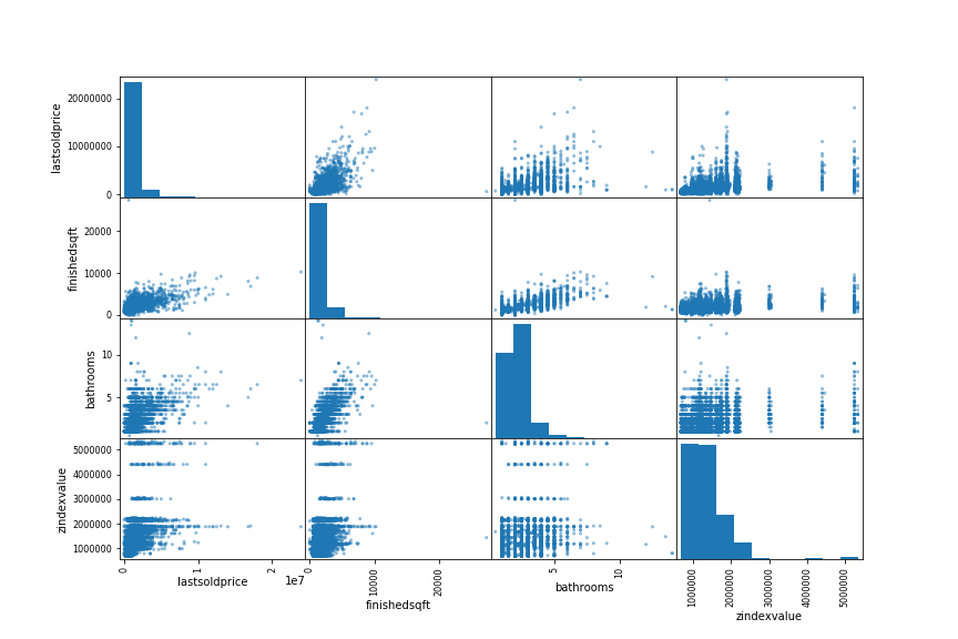
The most promising variable for predicting the last sold price is the finished sqft, so let’s zoom in on their correlation scatter plot.
sf.plot(kind="scatter", x="finishedsqft", y="lastsoldprice", alpha=0.5)
plt.savefig('scatter.png')
Gives this plot:
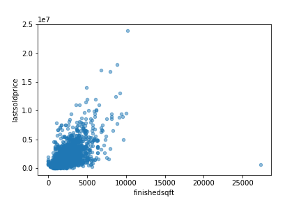
The correlation is indeed very strong; you can clearly see the upward trend and that the points are not too dispersed.
Because each house has different square footage and each neighborhood has different home prices, what we really need is the price per sqft. So, we add a new variable “price_per_sqft”. We then check to see how much this new independent variable correlates with the last sold price.
sf['price_per_sqft'] = sf['lastsoldprice']/sf['finishedsqft']

corr_matrix = sf.corr()
corr_matrix["lastsoldprice"].sort_values(ascending=False)
lastsoldprice     1.000000
finishedsqft      0.647208
bathrooms         0.536880
zindexvalue       0.460429
bedrooms          0.395478
latitude          0.283107
totalrooms        0.093527
price_per_sqft    0.005008
longitude        -0.052595
yearbuilt        -0.189055
Name: lastsoldprice, dtype: float64
Unfortunately, the new price_per_sqft variable shows only a very small positive correlation with the last sold price. But we still need this variable for grouping neighborhoods.
There are 71 neighborhoods in the data, and we are going to group them.
len(sf['neighborhood'].value_counts())
71
The following steps cluster the neighborhood into three groups: 1. low price; 2. high price low frequency; 3. high price high frequency.
freq = sf.groupby('neighborhood').count()['address']
mean = sf.groupby('neighborhood').mean()['price_per_sqft']
cluster = pd.concat([freq, mean], axis=1)
cluster['neighborhood'] = cluster.index
cluster.columns = ['freq', 'price_per_sqft','neighborhood']
cluster.describe()
Gives this table:
These are the low price neighborhoods:
cluster1 = cluster[cluster.price_per_sqft < 756]
cluster1.index
Index(['Bayview', 'Central Richmond', 'Central Sunset', 'Crocker Amazon',
       'Daly City', 'Diamond Heights', 'Excelsior', 'Forest Hill',
       'Forest Hill Extension', 'Golden Gate Heights', 'Ingleside',
       'Ingleside Heights', 'Ingleside Terrace', 'Inner Parkside',
       'Inner Richmond', 'Inner Sunset', 'Lakeshore', 'Little Hollywood',
       'Merced Heights', 'Mission Terrace', 'Mount Davidson Manor',
       'Oceanview', 'Outer Mission', 'Outer Parkside', 'Outer Richmond',
       'Outer Sunset', 'Parkside', 'Portola', 'Silver Terrace', 'Sunnyside',
       'Visitacion Valley', 'West Portal', 'Western Addition',
       'Westwood Highlands', 'Westwood Park'],
      dtype='object', name='neighborhood')
These are the high price and low frequency neighborhoods:
cluster_temp = cluster[cluster.price_per_sqft >= 756]
cluster2 = cluster_temp[cluster_temp.freq <123]
cluster2.index
Index(['Buena Vista Park', 'Central Waterfront - Dogpatch', 'Corona Heights',
       'Haight-Ashbury', 'Lakeside', 'Lone Mountain', 'Midtown Terrace',
       'North Beach', 'North Waterfront', 'Parnassus - Ashbury',
       'Presidio Heights', 'Sea Cliff', 'St. Francis Wood', 'Telegraph Hill',
       'Twin Peaks'],
      dtype='object', name='neighborhood')
These are the high price and high frequency neighborhoods:
cluster3 = cluster_temp[cluster_temp.freq >=123]
cluster3.index
Index(['Bernal Heights', 'Cow Hollow', 'Downtown',
       'Eureka Valley - Dolores Heights - Castro', 'Glen Park', 'Hayes Valley',
       'Lake', 'Lower Pacific Heights', 'Marina', 'Miraloma Park', 'Mission',
       'Nob Hill', 'Noe Valley', 'North Panhandle', 'Pacific Heights',
       'Potrero Hill', 'Russian Hill', 'South Beach', 'South of Market',
       'Van Ness - Civic Center', 'Yerba Buena'],
      dtype='object', name='neighborhood')
We add a group column based on the clusters:
def get_group(x):
    if x in cluster1.index:
        return 'low_price'
    elif x in cluster2.index:
        return 'high_price_low_freq'
    else:
        return 'high_price_high_freq'
sf['group'] = sf.neighborhood.apply(get_group)
After performing the above pre-processing, we do not need the following columns anymore: “address, lastsolddate, latitude, longitude, neighborhood, price_per_sqft”, so we drop them from our analysis.
sf.drop(sf.columns[[0, 4, 6, 7, 8, 13]], axis=1, inplace=True)
sf = sf[['bathrooms', 'bedrooms', 'finishedsqft', 'totalrooms', 'usecode', 'yearbuilt','zindexvalue', 'group', 'lastsoldprice']]
sf.head()
Gives this table:
Our data looks perfect!
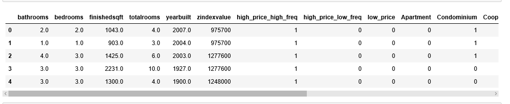
But before we build the model, we need to create dummy variables for these two categorical variables: “usecode” and “group”.
X = sf[['bathrooms', 'bedrooms', 'finishedsqft', 'totalrooms', 'usecode', 'yearbuilt', 'zindexvalue', 'group']]
Y = sf['lastsoldprice']

n = pd.get_dummies(sf.group)
X = pd.concat([X, n], axis=1)
m = pd.get_dummies(sf.usecode)
X = pd.concat([X, m], axis=1)
drops = ['group', 'usecode']
X.drop(drops, inplace=True, axis=1)
X.head()
Gives this table:
Train and Build a Linear Regression Model
from sklearn.cross_validation import train_test_split

X_train, X_test, y_train, y_test = train_test_split(X, Y, test_size=0.3, random_state=0)

from sklearn.linear_model import LinearRegression
regressor = LinearRegression()
regressor.fit(X_train, y_train)
LinearRegression(copy_X=True, fit_intercept=True, n_jobs=1, normalize=False)
Done! We now have a working Linear Regression model.
Calculate R squared:
y_pred = regressor.predict(X_test)
print('Liner Regression R squared: %.4f' % regressor.score(X_test, y_test))
Liner Regression R squared: 0.5619
So, in our model, 56.19% of the variability in Y can be explained using X. This is not that exciting.
Calculate root-mean-square error (RMSE):
import numpy as np
from sklearn.metrics import mean_squared_error
lin_mse = mean_squared_error(y_pred, y_test)
lin_rmse = np.sqrt(lin_mse)
print('Liner Regression RMSE: %.4f' % lin_rmse)
Liner Regression RMSE: 616071.5748
Our model was able to predict the value of every house in the test set within $616071 of the real price.
Calculate mean absolute error (MAE):
from sklearn.metrics import mean_absolute_error

lin_mae = mean_absolute_error(y_pred, y_test)
print('Liner Regression MAE: %.4f' % lin_mae)
Liner Regression MAE: 363742.1631
Random Forest
Let’s try a more complex model to see whether results can be improved — the RandomForestRegressor:
from sklearn.ensemble import RandomForestRegressor

forest_reg = RandomForestRegressor(random_state=42)
forest_reg.fit(X_train, y_train)
RandomForestRegressor(bootstrap=True, criterion='mse', max_depth=None,
           max_features='auto', max_leaf_nodes=None,
           min_impurity_split=1e-07, min_samples_leaf=1,
           min_samples_split=2, min_weight_fraction_leaf=0.0,
           n_estimators=10, n_jobs=1, oob_score=False, random_state=42,
           verbose=0, warm_start=False)
print('Random Forest R squared": %.4f' % forest_reg.score(X_test, y_test))
Random Forest R squared": 0.6491
y_pred = forest_reg.predict(X_test)
forest_mse = mean_squared_error(y_pred, y_test)
forest_rmse = np.sqrt(forest_mse)
print('Random Forest RMSE: %.4f' % forest_rmse)
Random Forest RMSE: 551406.0926
Much better! Let’s try one more.
Gradient boosting
from sklearn import ensemble
from sklearn.ensemble import GradientBoostingRegressor
model = ensemble.GradientBoostingRegressor()
model.fit(X_train, y_train)
GradientBoostingRegressor(alpha=0.9, criterion='friedman_mse', init=None,
             learning_rate=0.1, loss='ls', max_depth=3, max_features=None,
             max_leaf_nodes=None, min_impurity_split=1e-07,
             min_samples_leaf=1, min_samples_split=2,
             min_weight_fraction_leaf=0.0, n_estimators=100,
             presort='auto', random_state=None, subsample=1.0, verbose=0,
             warm_start=False)
print('Gradient Boosting R squared": %.4f' % model.score(X_test, y_test))
Gradient Boosting R squared": 0.6616
y_pred = model.predict(X_test)
model_mse = mean_squared_error(y_pred, y_test)
model_rmse = np.sqrt(model_mse)
print('Gradient Boosting RMSE: %.4f' % model_rmse)
Gradient Boosting RMSE: 541503.7962
These are the best results we got so far, so, I would consider this is our final model.
Feature Importance
We have used 19 features (variables) in our model. Let’s find out which features are important and vice versa.
feature_labels = np.array(['bathrooms', 'bedrooms', 'finishedsqft', 'totalrooms', 'yearbuilt', 'zindexvalue',
                           'high_price_high_freq', 'high_price_low_freq', 'low_price', 'Apartment', 'Condominium', 'Cooperative',
                          'Duplex', 'Miscellaneous', 'Mobile', 'MultiFamily2To4', 'MultiFamily5Plus', 'SingleFamily',
                           'Townhouse'])
importance = model.feature_importances_
feature_indexes_by_importance = importance.argsort()
for index in feature_indexes_by_importance:
    print('{}-{:.2f}%'.format(feature_labels[index], (importance[index] *100.0)))
Apartment-0.00%
MultiFamily5Plus-0.00%
Mobile-0.00%
Miscellaneous-0.00%
Cooperative-0.00%
Townhouse-0.00%
Condominium-0.54%
high_price_low_freq-0.69%
Duplex-1.21%
MultiFamily2To4-1.68%
high_price_high_freq-3.15%
bedrooms-3.17%
low_price-3.57%
SingleFamily-4.12%
yearbuilt-8.84%
totalrooms-9.13%
bathrooms-14.92%
zindexvalue-16.03%
finishedsqft-32.94%
The most important features are finished sqft, zindex value, number of bathrooms, total rooms, year built and so on. And the least important feature is Apartment, which means that regardless of whether this unit is an apartment or not, does not matter to the sold price. Overall, most of these 19 features are used.
Your Turn!
Hopefully, this post gives you a good idea of what a machine learning regression project looks like. As you can see, much of the work is in the data wrangling and the preparation steps, and these procedures consume most of the time spent on machine learning.
Now it’s time to get out there and start exploring and cleaning your data Try two or three algorithms, and let me know how it goes.