When it comes to finding out who your best customers are, the old RFM matrix principle is the best. RFM stands for Recency, Frequency, and Monetary. It is a customer segmentation technique that uses past purchase behavior to divide customers into groups.
RFM Score Calculations
RECENCY (R): Days since last purchase
FREQUENCY (F): Total number of purchases
MONETARY VALUE (M): Total money this customer spent
The Process
Step 1: Calculate the RFM metrics for each customer.
Step 2: Add segment numbers to RFM table.
Step 3: Sort according to the RFM scores from the best customers (score 111).
Since RFM is based on user activity data, the first thing we need is data.
Data
The dataset we will use is the same as when we did Market Basket Analysis — Online retail data set that can be downloaded from UCI Machine Learning Repository.
import pandas as pd
import warnings
warnings.filterwarnings('ignore')
df = pd.read_excel("Online_Retail.xlsx")
df.head()
df1 = df
The dataset contains all the transactions occurring between 01/12/2010 and 09/12/2011 for a UK-based and registered online retailer.
It took a few minutes to load the data, so I kept a copy as a backup.
Explore the data — validation and new variables
1. Missing values in important columns;
2. Customers’ distribution in each country;
3. Unit price and Quantity should > 0;
4. Invoice date should < today.
There were 38 unique countries as follows:
df1.Country.nunique()
df1.Country.unique()
38
array(['United Kingdom', 'France', 'Australia', 'Netherlands', 'Germany',
       'Norway', 'EIRE', 'Switzerland', 'Spain', 'Poland', 'Portugal',
       'Italy', 'Belgium', 'Lithuania', 'Japan', 'Iceland',
       'Channel Islands', 'Denmark', 'Cyprus', 'Sweden', 'Austria',
       'Israel', 'Finland', 'Bahrain', 'Greece', 'Hong Kong', 'Singapore',
       'Lebanon', 'United Arab Emirates', 'Saudi Arabia', 'Czech Republic',
       'Canada', 'Unspecified', 'Brazil', 'USA', 'European Community',
       'Malta', 'RSA'], dtype=object)
customer_country=df1[['Country','CustomerID']].drop_duplicates()
customer_country.groupby(['Country'])['CustomerID'].aggregate('count').reset_index().sort_values('CustomerID', ascending=False)
Country
CustomerID
36
United Kingdom
3950
14
Germany
95
13
France
87
31
....
More than 90% of the customers in the data are from the United Kingdom. There’s some research indicating that customer clusters vary by geography, so I’ll restrict the data to the United Kingdom only.
df1 = df1.loc[df1['Country'] == 'United Kingdom']
Check whether there are missing values in each column.
df1.isnull().sum(axis=0)
InvoiceNo           0
StockCode           0
Description      1454
Quantity            0
InvoiceDate         0
UnitPrice           0
CustomerID     133600
Country             0
dtype: int64
There are 133,600 missing values in the CustomerID column, and since our analysis is based on customers, we will remove these missing values.
df1 = df1[pd.notnull(df1['CustomerID'])]
Check the minimum values in UnitPrice and Quantity columns.
df1 = df1[pd.notnull(df1['CustomerID'])]
0.0
df1.Quantity.min()
-80995
Remove the negative values in Quantity column.
df1 = df1[(df1['Quantity']>0)]
df1.shape
df1.info()
(354345, 8)

Int64Index: 354345 entries, 0 to 541893
Data columns (total 8 columns):
InvoiceNo      354345 non-null object
StockCode      354345 non-null object
Description    354345 non-null object
Quantity       354345 non-null int64
InvoiceDate    354345 non-null datetime64[ns]
UnitPrice      354345 non-null float64
CustomerID     354345 non-null float64
Country        354345 non-null object
dtypes: datetime64[ns](1), float64(2), int64(1), object(4)
memory usage: 24.3+ MB
After cleaning up the data, we are now dealing with 354,345 rows and 8 columns.
Check unique value for each column.
def unique_counts(df1):
   for i in df1.columns:
       count = df1[i].nunique()
       print(i, ": ", count)
unique_counts(df1)
InvoiceNo :  16649
StockCode :  3645
Description :  3844
Quantity :  294
InvoiceDate :  15615
UnitPrice :  403
CustomerID :  3921
Country :  1
Add a column for total price.
df1['TotalPrice'] = df1['Quantity'] * df1['UnitPrice']
Find out the first and last order dates in the data.
df1['InvoiceDate'].min()
df1['InvoiceDate'].max()
Timestamp('2010-12-01 08:26:00')
Timestamp('2011-12-09 12:49:00')
Since recency is calculated for a point in time, and the last invoice date is 2011–12–09, we will use 2011–12–10 to calculate recency.
import datetime as dt
NOW = dt.datetime(2011,12,10)
df1['InvoiceDate'] = pd.to_datetime(df1['InvoiceDate'])
RFM Customer Segmentation
RFM segmentation starts from here.
Create a RFM table and Calculate RFM metrics for each customer
rfmTable = df1.groupby('CustomerID').agg({'InvoiceDate': lambda x: (NOW - x.max()).days,
                                        'InvoiceNo': lambda x: len(x),
                                        'TotalPrice': lambda x: x.sum()})

rfmTable['InvoiceDate'] = rfmTable['InvoiceDate'].astype(int)
rfmTable.rename(columns={'InvoiceDate': 'recency',
                         'InvoiceNo': 'frequency',
                         'TotalPrice': 'monetary_value'}, inplace=True)
rfmTable.head()
Gives this table:
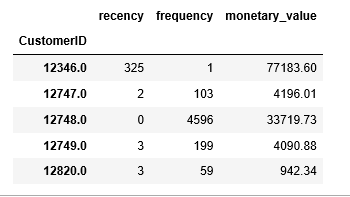
Interpretation:
- 1. CustomerID 12346 has frequency: 1, monetary value: $77,183.60 and recency: 325 days.
2. CustomerID 12747 has frequency: 103, monetary value: $4,196.01 and recency: 2 days
Let’s check the details of the first customer.
first_customer = df1[df1['CustomerID']== 12346.0]
first_customer
Gives this table:

The first customer has shopped only once, bought one product at a huge quantity(74,215). The unit price is very low; perhaps a clearance sale.
Split the metrics
The easiest way to split metrics into segments is by using quartiles.
- * This gives us a starting point for the detailed analysis.
* 4 segments are easy to understand and explain.
quantiles = rfmTable.quantile(q=[0.25,0.5,0.75])
quantiles = quantiles.to_dict()
Create a segmented RFM table
segmented_rfm = rfmTable
The lowest recency, highest frequency and monetary amounts are our best customers.
def RScore(x,p,d):
    if x <= d[p][0.25]:
        return 1
    elif x <= d[p][0.50]:
        return 2
    elif x <= d[p][0.75]:
        return 3
    else:
        return 4

def FMScore(x,p,d):
    if x <= d[p][0.25]:
        return 4
    elif x <= d[p][0.50]:
        return 3
    elif x <= d[p][0.75]:
        return 2
    else:
        return 1
Add segment numbers to the newly created segmented RFM table
segmented_rfm['r_quartile'] = segmented_rfm['recency'].apply(RScore, args=('recency',quantiles,))
segmented_rfm['f_quartile'] = segmented_rfm['frequency'].apply(FMScore, args=('frequency',quantiles,))
segmented_rfm['m_quartile'] = segmented_rfm['monetary_value'].apply(FMScore, args=('monetary_value',quantiles,))
segmented_rfm.head()
Gives this table:
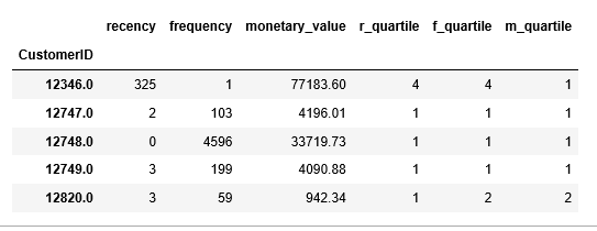
RFM segments split the customer base into an imaginary 3D cube which is hard to visualize. However, we can sort it out.
Add a new column to combine RFM score: 111 is the highest score as we determined earlier
segmented_rfm['RFMScore'] = segmented_rfm.r_quartile.map(str)
                            + segmented_rfm.f_quartile.map(str)
                            + segmented_rfm.m_quartile.map(str)
segmented_rfm.head()
Gives this table:
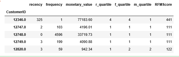
It is obvious that the first customer is not our best customer at all.
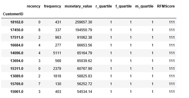
Who are the top 10 of our best customers!
segmented_rfm[segmented_rfm['RFMScore']=='111'].sort_values('monetary_value', ascending=False).head(10)
Gives this table:
Learn more
Interest to learn more?
- 1. Kimberly Coffey has an excellent tutorial on the same dataset using R.
2. Daniel McCarthy and Edward Wadsworth’s R package: Buy ’Til You Die — A Walkthrough.
3. Customer Segmentation for a wine seller from the yhat blog.
Source code that created this post can be found here. I would be pleased to receive feedback or questions on any of the above.
Reference: Blast Analytics and Marketing