Virtually everyone has had an online experience where a website makes personalized recommendations in hopes of future sales or ongoing traffic. Amazon tells you “Customers Who Bought This Item Also Bought”, Udemy tells you “Students Who Viewed This Course Also Viewed”. And Netflix awarded a $1 million prize to a developer team in 2009, for an algorithm that increased the accuracy of the company’s recommendation system by 10 percent.
Without further ado, if you want to learn how to build a recommender system from scratch, let’s get started.
The Data
Book-Crossings is a book rating dataset compiled by Cai-Nicolas Ziegler. It contains 1.1 million ratings of 270,000 books by 90,000 users. The ratings are on a scale from 1 to 10.
The data consists of three tables: ratings, books info, and users info. I downloaded these three tables from here.
import pandas as pd
import numpy as np
import matplotlib.pyplot as plt
books = pd.read_csv('BX-Books.csv', sep=';', error_bad_lines=False, encoding="latin-1")
books.columns = ['ISBN', 'bookTitle', 'bookAuthor', 'yearOfPublication', 'publisher', 'imageUrlS', 'imageUrlM', 'imageUrlL']
users = pd.read_csv('BX-Users.csv', sep=';', error_bad_lines=False, encoding="latin-1")
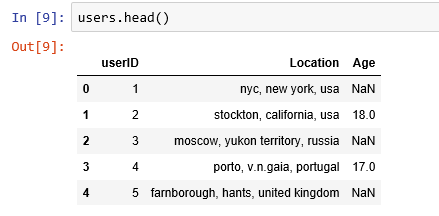
users.columns = ['userID', 'Location', 'Age']
ratings = pd.read_csv('BX-Book-Ratings.csv', sep=';', error_bad_lines=False, encoding="latin-1")
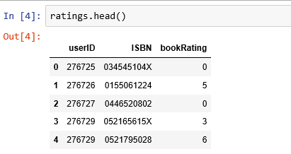
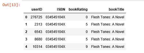
ratings.columns = ['userID', 'ISBN', 'bookRating']
Ratings data
The ratings data set provides a list of ratings that users have given to books. It includes 1,149,780 records and 3 fields: userID, ISBN, and bookRating.
print(ratings.shape)
print(list(ratings.columns))
(1149780, 3)
['userID', 'ISBN', 'bookRating']
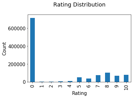
Ratings distribution
The ratings are very unevenly distributed, and the vast majority of ratings are 0.
plt.rc("font", size=15)
ratings.bookRating.value_counts(sort=False).plot(kind='bar')
plt.title('Rating Distribution\n')
plt.xlabel('Rating')
plt.ylabel('Count')
plt.savefig('system1.png', bbox_inches='tight')
plt.show()
Books data
The books dataset provides book details. It includes 271,360 records and 8 fields: ISBN, book title, book author, publisher and so on.
print(books.shape)
print(list(books.columns))
(271360, 8)
['ISBN', 'bookTitle', 'bookAuthor', 'yearOfPublication', 'publisher', 'imageUrlS', 'imageUrlM', 'imageUrlL']

Users data
This dataset provides the user demographic information. It includes 278,858 records and 3 fields: user id, location, and age.
print(users.shape)
print(list(users.columns))
(278858, 3)
['userID', 'Location', 'Age']
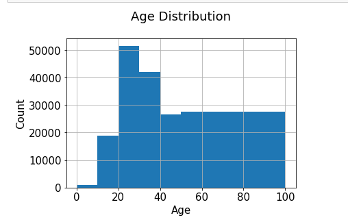
Age distribution
The most active users are among those in their 20–30s.
users.Age.hist(bins=[0, 10, 20, 30, 40, 50, 100])
plt.title('Age Distribution\n')
plt.xlabel('Age')
plt.ylabel('Count')
plt.savefig('system2.png', bbox_inches='tight')
plt.show()
Recommendations based on rating counts
rating_count = pd.DataFrame(ratings.groupby('ISBN')['bookRating'].count())
rating_count.sort_values('bookRating', ascending=False).head()
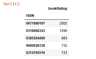
The book with ISBN “0971880107” received the most rating counts. Let’s find out what book it is, and what books are in the top 5.
most_rated_books = pd.DataFrame(['0971880107', '0316666343', '0385504209', '0060928336', '0312195516'], index=np.arange(5), columns = ['ISBN'])
most_rated_books_summary = pd.merge(most_rated_books, books, on='ISBN')
most_rated_books_summary
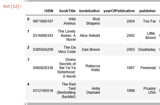
The book that received the most rating counts in this data set is Rich Shapero’s “Wild Animus”. And there is something in common among these five books that received the most rating counts — they are all novels. The recommender suggests that novels are popular and likely receive more ratings. And if someone likes “The Lovely Bones: A Novel”, we should probably also recommend to him(or her) “Wild Animus”.
Recommendations based on correlations
We use Pearsons’R correlation coefficient to measure the linear correlation between two variables, in our case, the ratings for two books.
First, we need to find out the average rating, and the number of ratings each book received.
average_rating = pd.DataFrame(ratings.groupby('ISBN')['bookRating'].mean())
average_rating['ratingCount'] = pd.DataFrame(ratings.groupby('ISBN')['bookRating'].count())
average_rating.sort_values('ratingCount', ascending=False).head()
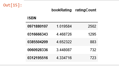
Observations: In this data set, the book that received the most rating counts was not highly rated at all. As a result, if we were to use recommendations based on rating counts, we would definitely make mistakes here. So, we need to have a better system.
To ensure statistical significance, users with less than 200 ratings, and books with less than 100 ratings are excluded.
counts1 = ratings['userID'].value_counts()
ratings = ratings[ratings['userID'].isin(counts1[counts1 >= 200].index)]
counts = ratings['bookRating'].value_counts()
ratings = ratings[ratings['bookRating'].isin(counts[counts >= 100].index)]
Rating matrix
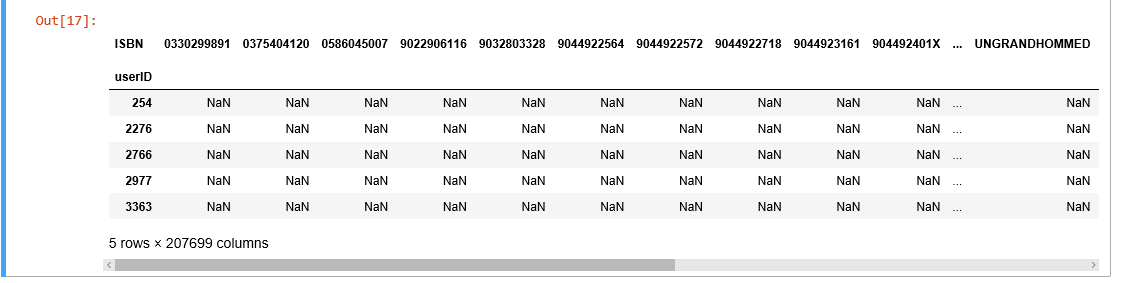
We convert the ratings table to a 2D matrix. The matrix will be sparse because not every user rated every book.
ratings_pivot = ratings.pivot(index='userID', columns='ISBN').bookRating
userID = ratings_pivot.index
ISBN = ratings_pivot.columns
print(ratings_pivot.shape)
ratings_pivot.head()
(905, 207699)
Let’s find out which books are correlated with the 2nd most rated book “The Lovely Bones: A Novel”.
To quote from Wikipedia: “It is the story of a teenage girl who, after being raped and murdered, watches from her personal Heaven as her family and friends struggle to move on with their lives while she comes to terms with her own death”.
bones_ratings = ratings_pivot['0316666343']
similar_to_bones = ratings_pivot.corrwith(bones_ratings)
corr_bones = pd.DataFrame(similar_to_bones, columns=['pearsonR'])
corr_bones.dropna(inplace=True)
corr_summary = corr_bones.join(average_rating['ratingCount'])
corr_summary[corr_summary['ratingCount']>=300].sort_values('pearsonR', ascending=False).head(10)
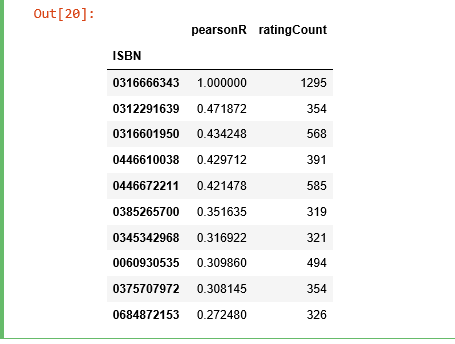
We obtained the books’ ISBNs, but we need to find out the titles of the books to see whether they make sense.
books_corr_to_bones = pd.DataFrame(['0312291639', '0316601950', '0446610038', '0446672211', '0385265700', '0345342968', '0060930535', '0375707972', '0684872153'],
                                  index=np.arange(9), columns=['ISBN'])
corr_books = pd.merge(books_corr_to_bones, books, on='ISBN')
corr_books

Let’s select three books from the above highly correlated list to examine: “The Nanny Diaries: A Novel”, “The Pilot’s Wife: A Novel” and “Where the Heart is”.
“The Nanny Diaries” satirizes upper-class Manhattan society as seen through the eyes of their children’s caregivers.
Written by the same author as “The Lovely Bones”, “The Pilot’s Wife” is the third novel in Shreve’s informal trilogy to be set in a large beach house on the New Hampshire coast that used to be a convent.
“Where the Heart Is” dramatizes in detail the tribulations of lower-income and foster children in the United States.
These three books sound like they would be highly correlated with “The Lovely Bones”. It seems our correlation recommender system is working.
Collaborative Filtering Using k-Nearest Neighbors (kNN)
kNN is a machine learning algorithm to find clusters of similar users based on common book ratings, and make predictions using the average rating of top-k nearest neighbors. For example, we first present ratings in a matrix with the matrix having one row for each item (book) and one column for each user, like so:
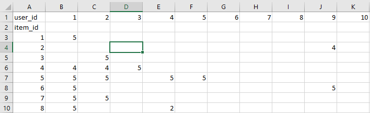
We then find the k item that has the most similar user engagement vectors. In this case, Nearest Neighbors of item id 5= [7, 4, 8, …]. Now, let’s implement kNN into our book recommender system.
Starting from the original data set, we will be only looking at the popular books. In order to find out which books are popular, we combine books data with ratings data.
combine_book_rating = pd.merge(ratings, books, on='ISBN')
columns = ['yearOfPublication', 'publisher', 'bookAuthor', 'imageUrlS', 'imageUrlM', 'imageUrlL']
combine_book_rating = combine_book_rating.drop(columns, axis=1)
combine_book_rating.head()
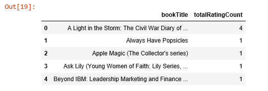
We then group by book titles and create a new column for total rating count.
combine_book_rating = combine_book_rating.dropna(axis = 0, subset = ['bookTitle'])

book_ratingCount = (combine_book_rating.
     groupby(by = ['bookTitle'])['bookRating'].
     count().
     reset_index().
     rename(columns = {'bookRating': 'totalRatingCount'})
     [['bookTitle', 'totalRatingCount']]
    )
book_ratingCount.head()
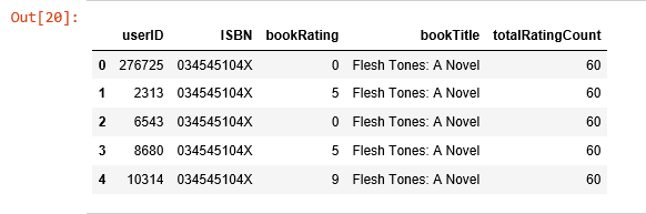
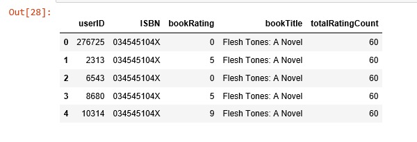
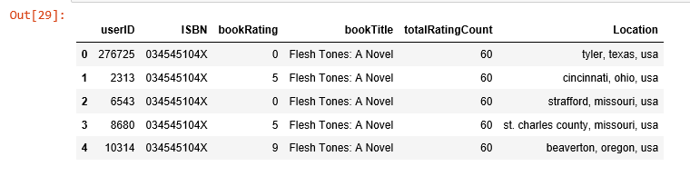
We combine the rating data with the total rating count data, this gives us exactly what we need to find out which books are popular and filter out lesser-known books.
rating_with_totalRatingCount = combine_book_rating.merge(book_ratingCount, left_on = 'bookTitle', right_on = 'bookTitle', how = 'left')
rating_with_totalRatingCount.head()
Let’s look at the statistics of total rating count:
pd.set_option('display.float_format', lambda x: '%.3f' % x)
print(book_ratingCount['totalRatingCount'].describe())
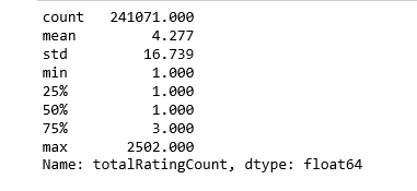
The median book has been rated only once. Let’s look at the top of the distribution:
print(book_ratingCount['totalRatingCount'].quantile(np.arange(.9, 1, .01)))
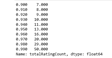
About 1% of the books received 50 or more ratings. Because we have so many books in our data, we will limit it to the top 1%, and this will give us 2713 unique books.
popularity_threshold = 50
rating_popular_book = rating_with_totalRatingCount.query('totalRatingCount >= @popularity_threshold')
rating_popular_book.head()
Filter to users in US and Canada only
In order to improve computing speed, and not run into the “MemoryError” issue, I will limit our user data to those in the US and Canada. And then combine user data with the rating data and total rating count data.
combined = rating_popular_book.merge(users, left_on = 'userID', right_on = 'userID', how = 'left')

us_canada_user_rating = combined[combined['Location'].str.contains("usa|canada")]
us_canada_user_rating=us_canada_user_rating.drop('Age', axis=1)
us_canada_user_rating.head()
Implementing kNN
We convert our table to a 2D matrix, and fill the missing values with zeros (since we will calculate distances between rating vectors). We then transform the values(ratings) of the matrix dataframe into a scipy sparse matrix for more efficient calculations.
Finding the Nearest Neighbors
We use unsupervised algorithms with sklearn.neighbors. The algorithm we use to compute the nearest neighbors is “brute”, and we specify “metric=cosine” so that the algorithm will calculate the cosine similarity between rating vectors. Finally, we fit the model.
us_canada_user_rating = us_canada_user_rating.drop_duplicates(['userID', 'bookTitle'])
us_canada_user_rating_pivot = us_canada_user_rating.pivot(index = 'bookTitle', columns = 'userID', values = 'bookRating').fillna(0)
us_canada_user_rating_matrix = csr_matrix(us_canada_user_rating_pivot.values)

from sklearn.neighbors import NearestNeighbors

model_knn = NearestNeighbors(metric = 'cosine', algorithm = 'brute')
model_knn.fit(us_canada_user_rating_matrix)
NearestNeighbors(algorithm='brute', leaf_size=30, metric='cosine',
         metric_params=None, n_jobs=1, n_neighbors=5, p=2, radius=1.0)
Test our model and make some recommendations:
In this step, the kNN algorithm measures distance to determine the “closeness” of instances. It then classifies an instance by finding its nearest neighbors, and picks the most popular class among the neighbors.
query_index = np.random.choice(us_canada_user_rating_pivot.shape[0])
distances, indices = model_knn.kneighbors(us_canada_user_rating_pivot.iloc[query_index, :].reshape(1, -1), n_neighbors = 6)

for i in range(0, len(distances.flatten())):
    if i == 0:
        print('Recommendations for {0}:\n'.format(us_canada_user_rating_pivot.index[query_index]))
    else:
        print('{0}: {1}, with distance of {2}:'.format(i, us_canada_user_rating_pivot.index[indices.flatten()[i]], distances.flatten()[i]))
Recommendations for the Green Mile: Coffey's Hands (Green Mile Series):

1: The Green Mile: Night Journey (Green Mile Series), with distance of 0.26063737394209996:
2: The Green Mile: The Mouse on the Mile (Green Mile Series), with distance of 0.2911623754404248:
3: The Green Mile: The Bad Death of Eduard Delacroix (Green Mile Series), with distance of 0.2959542871302775:
4: The Two Dead Girls (Green Mile Series), with distance of 0.30596709534565514:
5: The Green Mile: Coffey on the Mile (Green Mile Series), with distance of 0.37646848777592923:
Perfect! Green Mile Series books definitely should be recommended, one after another.
Collaborative Filtering Using Matrix Factorization
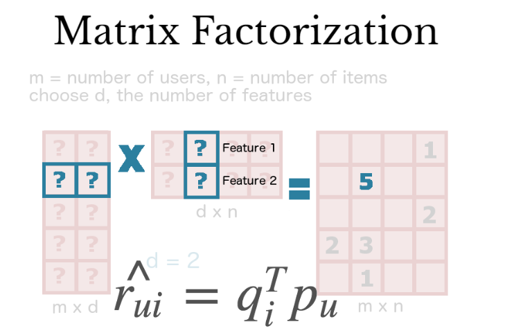
Matrix Factorization is simply a mathematical tool for playing around with matrices. The Matrix Factorization techniques are usually more effective, because they allow users to discover the latent (hidden)features underlying the interactions between users and items (books).
We use singular value decomposition (SVD) — one of the Matrix Factorization models for identifying latent factors.
Similar with kNN, we convert our USA Canada user rating table into a 2D matrix (called a utility matrix here) and fill the missing values with zeros.
us_canada_user_rating_pivot2 = us_canada_user_rating.pivot(index = 'userID', columns = 'bookTitle', values = 'bookRating').fillna(0)
us_canada_user_rating_pivot2.head()
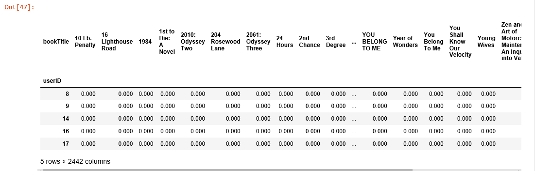
We then transpose this utility matrix, so that the bookTitles become rows and userIDs become columns. After using TruncatedSVD to decompose it, we fit it into the model for dimensionality reduction. This compression happened on the dataframe’s columns since we must preserve the book titles. We choose n_components = 12 for just 12 latent variables, and you can see, our data’s dimensions have been reduced significantly from 40017 X 2442 to 2442 X 12.
us_canada_user_rating_pivot2.shape
(40017, 2442)
X = us_canada_user_rating_pivot2.values.T
X.shape
(2442, 40017)
import sklearn
from sklearn.decomposition import TruncatedSVD

SVD = TruncatedSVD(n_components=12, random_state=17)
matrix = SVD.fit_transform(X)
matrix.shape
(2442, 12)
We calculate the Pearson’s R correlation coefficient for every book pair in our final matrix. To compare this with the results from kNN, we pick the same book “The Green Mile: Coffey’s Hands (Green Mile Series)” to find the books that have high correlation coefficients (between 0.9 and 1.0) with it.
import warnings
warnings.filterwarnings("ignore",category =RuntimeWarning)
corr = np.corrcoef(matrix)
corr.shape
(2442, 2442)
us_canada_book_title = us_canada_user_rating_pivot2.columns
us_canada_book_list = list(us_canada_book_title)
coffey_hands = us_canada_book_list.index("The Green Mile: Coffey's Hands (Green Mile Series)")
print(coffey_hands)
1906
There you have it!
corr_coffey_hands  = corr[coffey_hands]
list(us_canada_book_title[(corr_coffey_hands0.9)])
['Needful Things',
 'The Bachman Books: Rage, the Long Walk, Roadwork, the Running Man',
 'The Green Mile: Coffey on the Mile (Green Mile Series)',
 'The Green Mile: Night Journey (Green Mile Series)',
 'The Green Mile: The Bad Death of Eduard Delacroix (Green Mile Series)',
 'The Green Mile: The Mouse on the Mile (Green Mile Series)',
 'The Shining',
 'The Two Dead Girls (Green Mile Series)']
Not too shabby! Our system can beat Amazon’s, what do you think?
References:
- Music Recommendations
ohAI