This exercise focuses on linear regression with both analytical (normal equation) and numerical (gradient descent) methods. We will start with linear regression with one variable. From this part of the exercise, we will create plots that help to visualize how gradient descent gets the coefficient of the predictor and the intercept. In the second part, we will implement linear regression with multiple variables.
Linear regression with one variable
In this part of this exercise, we will implement linear regression with one variable to predict profits for a food truck. Suppose you are the CEO of a restaurant franchise and are considering different cities for opening a new outlet. The chain already has trucks in various cities and you have data for profits and populations from cities. We would like to use this data to help us select which city to expand to next.
The file ex1data1.txt contains the dataset for our linear regression problem. The first column is the population of a city and the second column is the profit of a food truck in that city. A negative value for profit indicates a loss. The first column refers to the population size in 10,000s and the second column refers to the profit in $10,000s.
library(ggplot2)
library(data.table)
library(magrittr)
library(caret)
library(fields)
library(plot3D)
Load the data and display first 6 observations
ex1data1 <- fread("ex1data1.txt",col.names=c("population","profit"))
head(ex1data1)
   population  profit
1:     6.1101 17.5920
2:     5.5277  9.1302
3:     8.5186 13.6620
4:     7.0032 11.8540
5:     5.8598  6.8233
6:     8.3829 11.8860
Plotting the Data
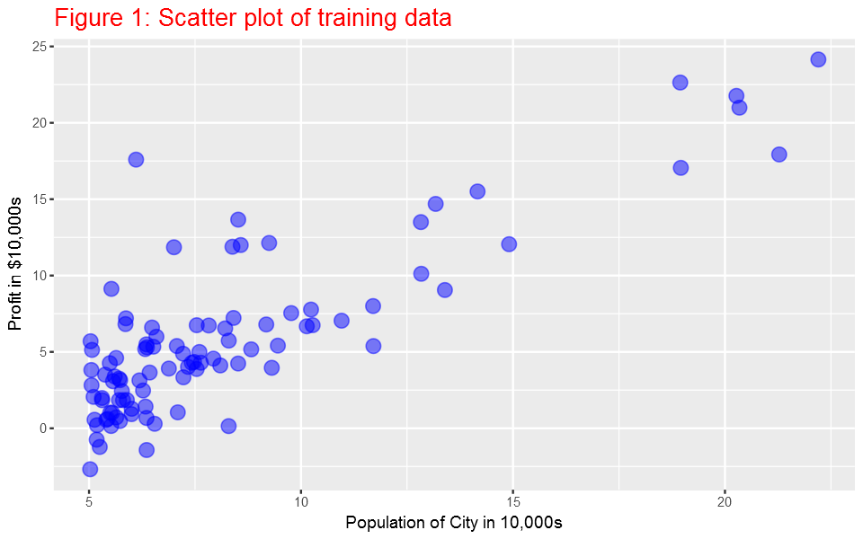
Before starting on any task, it is often useful to understand the data by visualizing it. For this dataset, we can use a scatter plot to visualize the data, since it has only two properties to plot (profit and population). Many other problems that we encounter in real life are multi-dimensional and can’t be plotted on a 2-d plot.
ex1data1%>%ggplot(aes(x=population, y=profit))+
geom_point(color="blue",size=4,alpha=0.5)+
ylab('Profit in $10,000s')+
xlab('Population of City in 10,000s')+ggtitle ('Figure 1: Scatter plot of training data')+
theme(plot.title = element_text(size = 16,colour="red"))
Here it is the plot:
Gradient Descent
In this part, we will fit linear regression parameters θ to our dataset using gradient descent.
To implement gradient descent, we need to calculate the cost, which is given by:
Computing the cost J(θ)
As we perform gradient descent to learn minimize the cost function J(θ), it is helpful to monitor the convergence by computing the cost. In this section, we will implement a function to calculate J(θ) so we can check the convergence of our gradient descent implementation.
But remember, before we go any further we need to add the θ intercept term.
X=cbind(1,ex1data1$population)
y=ex1data1$profit
head(X)
     [,1]   [,2]
[1,]    1 6.1101
[2,]    1 5.5277
[3,]    1 8.5186
[4,]    1 7.0032
[5,]    1 5.8598
[6,]    1 8.3829
The function below calcuates cost based on the equation given above.
computeCost=function(X,y,theta){
    z=((X%*%theta)-y)^2
    return(sum(z)/(2*nrow(X)))
}
Now, we can calculate the initial cost by initilizating the initial parameters to 0.
theta=matrix(rep(0,ncol(X)))
round(computeCost(X,y,theta),2)
32.07
Gradient descent
Next, we will implement gradient descent by calling the computeCost function above. A good way to verify that gradient descent is working correctly is to look at the value of J(θ) and check that it is decreasing with each step. Our value of J(θ) should never increase, and should converge to a steady value by the end of the algorithm.
The gradient descent function below returns the cost in every iteration and the optimal parameters for the number of iterations and learning rate alpha specified.
gradientDescent=function(X, y, theta, alpha, iters){
gd=list()
cost=rep(0,iters)
for(k in 1:iters){
  z=rep(0,ncol(X))
  for(i in 1:ncol(X)){
      for(j in 1:nrow(X)){
          z[i]=z[i]+(((X[j,]%*%theta)-y[j])*X[j,i])
          }
      }
theta= theta-((alpha/nrow(X))*z)
cost[k]=computeCost(X,y,theta)
    }
    gd$theta= theta
    gd$cost=cost
    gd
}
Now, let’s use the gradientDescent function to find the parameters and we have to make sure that our cost never increases. Let’s use 1500 iterations and a learning rate alpha of 0.04 for now. Later, we will see the effect of these values in our application.
iterations = 1500
alpha = 0.01
theta= matrix(rep(0, ncol(X)))
gradientDescent_results=gradientDescent(X,y,theta,alpha,iterations)
theta=gradientDescent_results$theta
theta
          [,1]
[1,] -3.630291
[2,]  1.166362
Ploting the cost function as a function of the number of iterations
We expect that the cost should be decreasing or at least should not be at all increasing if our implementaion is correct. Let’s plot the cost fucntion as a function of number of iterations and make sure our implemenation makes sense.
data.frame(Cost=gradientDescent_results$cost,Iterations=1:iterations)%>%
ggplot(aes(x=Iterations,y=Cost))+geom_line(color="blue")+
ggtitle("Cost as a function of number of iteration")+
theme(plot.title = element_text(size = 16,colour="red"))
Here it is the plot:
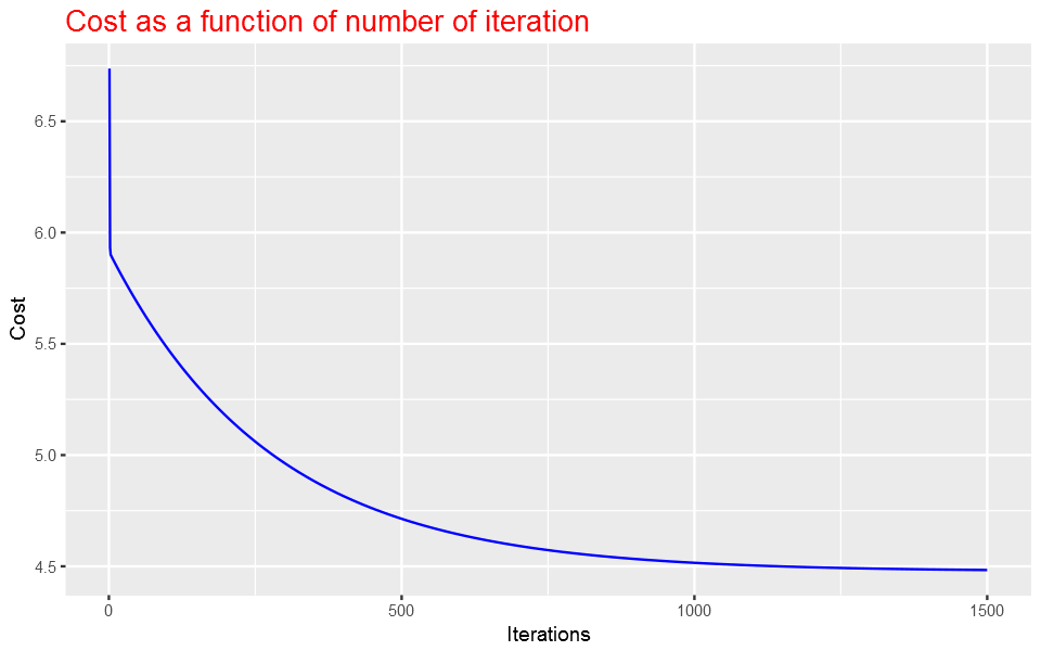
As the plot above shows, the cost decrases with number of iterations and gets almost close to convergence with 1500 iterations.
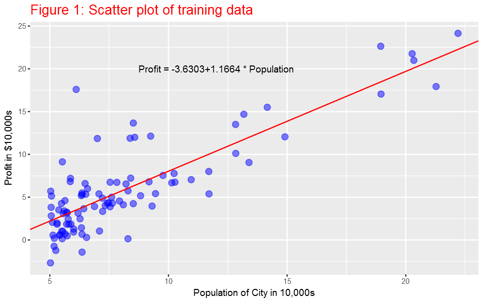
Plot the linear fit
Now, since we know the parameters (slope and intercept), we can plot the linear fit on the scatter plot.
ex1data1%>%ggplot(aes(x=population, y=profit))+
geom_point(color="blue",size=3,alpha=0.5)+
ylab('Profit in $10,000s')+
xlab('Population of City in 10,000s')+
ggtitle ('Figure 1: Scatter plot of training data') +
geom_abline(intercept = theta[1], slope = theta[2],col="red",show.legend=TRUE)+
theme(plot.title = element_text(size = 16,colour="red"))+
annotate("text", x = 12, y = 20, label = paste0("Profit = ",round(theta[1],4),"+",round(theta[2],4)," * Population"))
Here it is the plot:
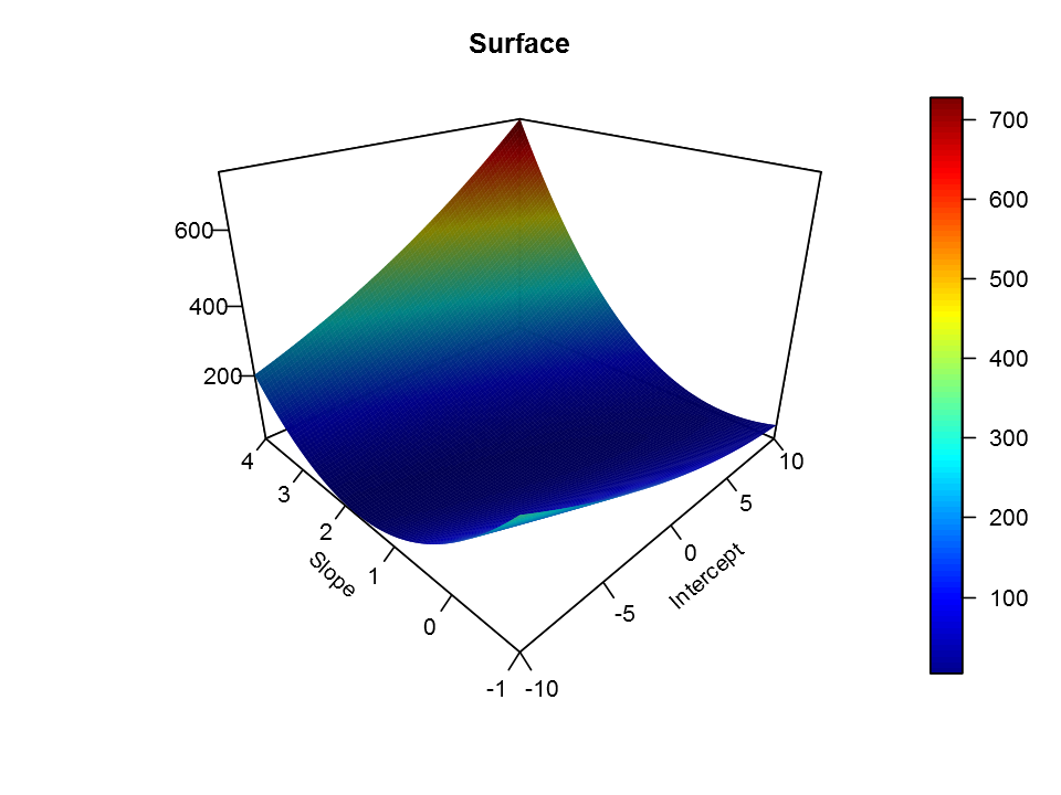
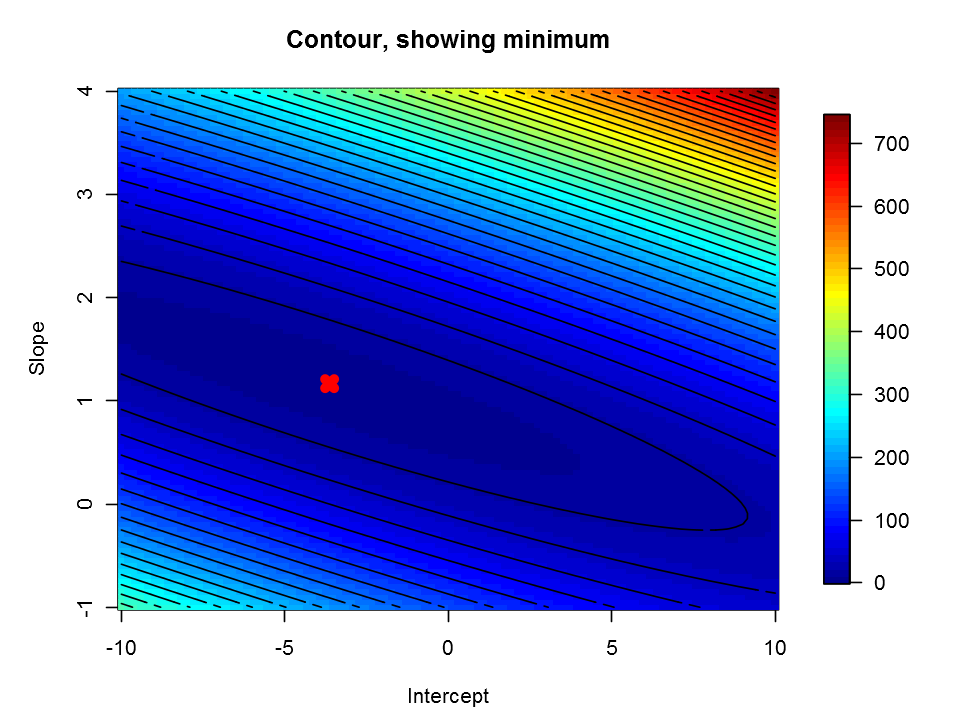
Visualizing J(θ)
To understand the cost function J(θ) better, let’s now plot the cost over a 2-dimensional grid of θ0 and θ1 values. The global minimum is the optimal point for θ0 and θ1, and each step of gradient descent moves closer to this point.
Intercept=seq(from=-10,to=10,length=100)
Slope=seq(from=-1,to=4,length=100)
# initialize cost values to a matrix of 0's
Cost = matrix(0,length(Intercept), length(Slope));
for(i in 1:length(Intercept)){
    for(j in 1:length(Slope)){
        t = c(Intercept[i],Slope[j])
        Cost[i,j]= computeCost(X, y, t)
    }
}
persp3D(Intercept,Slope,Cost,theta=-45, phi=25, expand=0.75,lighting = TRUE,
        ticktype="detailed", xlab="Intercept", ylab="Slope",
        zlab="",axes=TRUE, main="Surface")
image.plot(Intercept,Slope,Cost, main="Contour, showing minimum")
contour(Intercept,Slope,Cost, add = TRUE,n=30,labels='')
points(theta[1],theta[2],col='red',pch=4,lwd=6)
Here it is the plot:
Normal Equation
Since linear regression has closed-form solution, we can solve it analytically and it is called normal equation. It is given by the formula below. we do not need to iterate or choose learning curve. However, we need to calculate inverse of a matrix , which make it slow if the number of records is very large. Gradient descent is applicable to other machine learning techniques as well. Further, gradient descent method is more appropriate even to linear regression when the number of observations is very large.
θ=(XTX)−1XTy
theta2=solve((t(X)%*%X))%*%t(X)%*%y
theta2
          [,1]
[1,] -3.895781
[2,]  1.193034
There is very small difference between the parameters we got from normal equation and using gradient descent. Let’s increase the number of iteration and see if they get closer to each other. I increased the number of iterations from 1500 to 15000.
iterations = 15000
alpha = 0.01
theta= matrix(rep(0, ncol(X)))
gradientDescent_results=gradientDescent(X,y,theta,alpha,iterations)
theta=gradientDescent_results$theta
theta
          [,1]
[1,] -3.895781
[2,]  1.193034
As you can see, now the results from normal equation and gradient descent are the same.
Using caret package
By the way, we can use packages develoed by experts in the field and perform our machine learning tasks. There are many machine learning packages in R for differnt types of machine learning tasks. To verify that we get the same results, let’s use the caret package, which is among the most commonly used machine learning packages in R.
my_lm <- train(profit~population, data=ex1data1,method = "lm")
my_lm$finalModel$coefficients
(Intercept) -3.89578087831187
population  1.1930336441896
Linear regression with multiple variables
In this part of the exercise, we will implement linear regression with multiple variables to predict the prices of houses. Suppose you are selling your house and you want to know what a good market price would be. One way to do this is to first collect information on recent houses sold and make a model of housing prices. The file ex1data2.txt contains a training set of housing prices in Port- land, Oregon. The first column is the size of the house (in square feet), the second column is the number of bedrooms, and the third column is the price of the house.
ex1data2 <- fread("ex1data2.txt",col.names=c("size","bedrooms","price"))
head(ex1data2)
   size bedrooms  price
1: 2104        3 399900
2: 1600        3 329900
3: 2400        3 369000
4: 1416        2 232000
5: 3000        4 539900
6: 1985        4 299900
Feature Normalization
House sizes are about 1000 times the number of bedrooms. When features differ by orders of magnitude, first performing feature scaling can make gradient descent converge much more quickly.
ex1data2=as.data.frame(ex1data2)
for(i in 1:(ncol(ex1data2)-1)){
    ex1data2[,i]=(ex1data2[,i]-mean(ex1data2[,i]))/sd(ex1data2[,i])
}
Gradient Descent
Previously, we implemented gradient descent on a univariate regression problem. The only difference now is that there is one more feature in the matrix X. The hypothesis function and the batch gradient descent update rule remain unchanged.
X=cbind(1,ex1data2$size,ex1data2$bedrooms)
y=ex1data2$price
head(X)

iterations = 6000
alpha = 0.01
theta= matrix(rep(0, ncol(X)))
gradientDescent_results=gradientDescent(X,y,theta,alpha,iterations)
theta=gradientDescent_results$theta
theta
    [,1]        [,2]       [,3]
[1,]    1  0.13000987 -0.2236752
[2,]    1 -0.50418984 -0.2236752
[3,]    1  0.50247636 -0.2236752
[4,]    1 -0.73572306 -1.5377669
[5,]    1  1.25747602  1.0904165
[6,]    1 -0.01973173  1.0904165

          [,1]
[1,] 340412.660
[2,] 110631.050
[3,]  -6649.474
Normal Equation
theta2=solve((t(X)%*%X))%*%t(X)%*%y
theta2
           [,1]
[1,] 340412.660
[2,] 110631.050
[3,]  -6649.474
Using caret package
ex1data2 <- fread("ex1data2.txt",col.names=c("size","bedrooms","price"))
my_lm <- train(price~size+bedrooms, data=ex1data2,method = "lm",
               preProcess = c("center","scale"))
my_lm$finalModel$coefficients
(Intercept) 340412.659574468
size        110631.050278846
bedrooms  -6649.4742708198
Summary
In this post, we saw how to implement numerical and analytical solutions to linear regression problems using R. We also used caret -the famous R machine learning package- to verify our results. The data sets are from the Coursera machine learning course offered by Andrew Ng. The course is offered with Matlab/Octave. I am doing the exercises in that course with R. You can get the code from this Github repository.