Last time we discussed the conversion of longitudinal data between wide and long formats and visualised individual growth trajectories using a sample randomised controlled trial dataset. But could we take this a step farther and predict the trajectory of the outcomes over time?
Yes, of course! We could estimate that using multilevel growth models (also known as hierarchical models or mixed models).
Generate a longitudinal dataset and convert it into long format
Let’s start by remaking the dataset from my previous post:
library(MASS)

dat.tx.a <- mvrnorm(n=250, mu=c(30, 20, 28),
                    Sigma=matrix(c(25.0, 17.5, 12.3,
                                   17.5, 25.0, 17.5,
                                   12.3, 17.5, 25.0), nrow=3, byrow=TRUE))

dat.tx.b <- mvrnorm(n=250, mu=c(30, 20, 22),
                    Sigma=matrix(c(25.0, 17.5, 12.3,
                                   17.5, 25.0, 17.5,
                                   12.3, 17.5, 25.0), nrow=3, byrow=TRUE))

dat <- data.frame(rbind(dat.tx.a, dat.tx.b))
names(dat) <- c('measure.1', 'measure.2', 'measure.3')

dat <- data.frame(subject.id = factor(1:500), tx = rep(c('A', 'B'), each = 250), dat)

rm(dat.tx.a, dat.tx.b)

dat <- reshape(dat, varying = c('measure.1', 'measure.2', 'measure.3'),
               idvar = 'subject.id', direction = 'long')
Multilevel growth models
There are many R packages to help your to do multilevel analysis, but I find lme4 to be one of the best because of its simplicity and ability to fit generalised models (e.g. for binary and count outcomes). A popular alternative is the nlme package, which should provide similar results for continuous outcomes (with a normal/Gaussian distribution). So let’s start analysing the overall trend of the depression score.
# install.packages('lme4')
library(lme4)
m <- lmer(measure ~ time + (1 | subject.id), data = dat)
You should be very familiar with the syntax if you have done a linear regression before. Basically it’s just the lm() function with the additional random effect part in the formula.
Random effects, if you aren’t familiar with them, are basically any variation in our data that are outside of the experimenter’s control. So for instance, the treatment that a participant receives is a fixed effect because we as experimenters determine which patients receive treatment A and which receive treatment B. However, the baseline depression score at the start of treatment is likely going to vary from individual to individual: some will be more depressed; others less depressed. Since that’s out of our control, we’ll consider that a random effect.
Specifically, these differences in baseline depression scores represents a random intercept (i.e., different participants start off at different levels of depression). We can also have models with random slopes: for instance, if we have reason to believe that some participants might respond really well to treatment and others might only see a small benefit, despite coming in with similar levels of depression.
Using lmer‘s syntax, we specify a random intercept using the syntax DV ~ IV + (1 | rand.int) where DV is your outcome variable, IV represents your independent variables, 1 represents the coefficients (or slope) of your independent variables, and rand.int is the variable acting as a random intercept. Usually this will be a column of participant IDs.
Likewise, a random slopes model is specified using the syntax DV ~ IV + (rand.slope | rand.int).
Here are the results of the multilevel model using the summary() function:
summary(m)

Linear mixed model fit by REML ['lmerMod']
Formula: measure ~ time + (1 | subject.id)
   Data: dat

REML criterion at convergence: 9639.6

Scaled residuals:
     Min       1Q   Median       3Q      Max
-2.45027 -0.70596  0.00832  0.65951  2.78759

Random effects:
 Groups     Name        Variance Std.Dev.
 subject.id (Intercept)  9.289   3.048
 Residual               28.860   5.372
Number of obs: 1500, groups:  subject.id, 500

Fixed effects:
            Estimate Std. Error t value
(Intercept)  29.8508     0.3915   76.25
time         -2.2420     0.1699  -13.20

Correlation of Fixed Effects:
     (Intr)
time -0.868
(The REML criterion is an indicator for estimation convergence. Normally speaking you don’t need to be too worried about this because if there’s potential convergence problem in estimation, the lmer() will give you some warnings. )
The Random effects section of the results state the variance structure of the data. There are two sources of variance in this model: the residual (the usual one as in linear models) and the interpersonal difference (i.e. subject.id). One common way to quantify the strength of interpersonal difference is the intraclass correlation coefficient (ICC). It is possible to compute the ICC from the multilevel model and it is just \(\frac{9.289}{9.289 + 28.860} = 0.243\), which means 24.3% of the variation in depression score could be explained by interpersonal difference.
Let’s move to the Fixed effects section. Hmmm… Where are the p-values? Well, although SAS and other statistical software do provide p-values for fixed effects in multilevel models, their calculations are not a consensus among statisticians. To put it simplly, the degrees of freedom associated with these t-statistics are not well understood and without the degrees of freedom, we don’t know the exact distribution of the t-statistics and thus we don’t know the p-values. SAS and other programs have a workaround using approximation, which the developer of the lme4 package doesn’t feel very comfortable with. As a result, the lmer package intentionally does not report p-values in the results. (So don’t be afraid not to include them! There are other and arguably better measures of your model’s significance that we can use.)
That said, if p-values are absolutely required, we can approximate them with the lmerTest package which builds on top of lme4.
Multilevel growth models with approximate p-values
The code here is largely the same as above, except we’re now using the lmerTest package.
# install.packages('lme4')
# Please note the explanation and limitations:
# https://stat.ethz.ch/pipermail/r-help/2006-May/094765.html
library(lmerTest)
m <- lmer(measure ~ time + (1 | subject.id), data = dat)
The results are very similar, but now we got the approximate degrees of freedom and p-values. So we’re now confident in saying that the average participant of the RCT are now having decreasing depression score over time. The decrement is about 2.24 points for one time point.
summary(m)

Linear mixed model fit by REML t-tests
use Satterthwaite approximations to
degrees of freedom [merModLmerTest]
Formula: measure ~ time + (1 | subject.id)
   Data: dat

REML criterion at convergence: 9639.6

Scaled residuals:
     Min       1Q   Median       3Q      Max
-2.45027 -0.70596  0.00832  0.65951  2.78759

Random effects:
 Groups     Name        Variance Std.Dev.
 subject.id (Intercept)  9.289   3.048
 Residual               28.860   5.372
Number of obs: 1500, groups:  subject.id, 500

Fixed effects:
             Estimate Std. Error        df t value Pr(>|t|)
(Intercept)   29.8508     0.3915 1449.4000   76.25   <2e-16 ***
time          -2.2420     0.1699  999.0000  -13.20   <2e-16 ***
---
Signif. codes:  0 ‘***’ 0.001 ‘**’ 0.01 ‘*’ 0.05 ‘.’ 0.1 ‘ ’ 1

Correlation of Fixed Effects:
     (Intr)
time -0.868
Calculating 95% CI and PI
Sometimes we want to plot the average value on top of the individual trajectories. To show the uncertainty associated with the averages, we’d need to use the fitted model to calculate the fitted values, the 95% confidence intervals (CI), the 95% prediction intervals (PI).
# See for details: http://glmm.wikidot.com/faq
dat.new <- data.frame(time = 1:3)
dat.new$measure <- predict(m, dat.new, re.form = NA)

m.mat <- model.matrix(terms(m), dat.new)

dat.new$var <- diag(m.mat %*% vcov(m) %*% t(m.mat)) + VarCorr(m)$subject.id[1]
dat.new$pvar <- dat.new$var + sigma(m)^2
dat.new$ci.lb <- with(dat.new, measure - 1.96 * sqrt(var))
dat.new$ci.ub <- with(dat.new, measure + 1.96 * sqrt(var))
dat.new$pi.lb <- with(dat.new, measure - 1.96 * sqrt(pvar))
dat.new$pi.ub <- with(dat.new, measure + 1.96 * sqrt(pvar))
The first line of the code specifies the time points that we want the average values, which are simply time 1, 2, and 3 in our case. The second line uses the predict() function to get the average values from the model ignoring the conditional random effects (re.form = NA). Lines 3 and 4 calculate the variances of the average values: it’s basically the matrix cross-products plus the variance of the random intercept. Line 5 calculates the variances of a single observation, which is the variance of the average values plus the residual variance. Lines 6 to 9 are just the standard calculation of 95% CIs and PIs assuming normal distribution. This ends up giving us data to plot that look like:
dat.new

time  measure      var     pvar    ci.lb    ci.ub     pi.lb    pi.ub
   1 27.72421 10.85669 43.04054 21.26611 34.18231 14.865574 40.58285
   2 25.22342 10.82451 43.00835 18.77490 31.67194 12.369592 38.07725
   3 22.72263 10.85669 43.04054 16.26453 29.18073  9.863993 35.58127
Plot the average values
Finally, let’s plot the averages with 95% CIs and PIs. Notice that the PIs are much wider than the CIs. That means we’re much more confident in predicting the average than a single value.
ggplot(data = dat.new, aes(x = time, y = measure)) +
  geom_line(data = dat, alpha = .02, aes(group = subject.id)) +
  geom_errorbar(width = .02, colour = 'red',
                aes(x = time - .02, ymax = ci.ub, ymin = ci.lb)) +
  geom_line(colour = 'red', linetype = 'dashed', aes(x = time-.02)) +
  geom_point(size = 3.5, colour = 'red', fill = 'white', aes(x = time - .02)) +
  geom_errorbar(width = .02, colour = 'blue',
                aes(x = time + .02, ymax = pi.ub, ymin = pi.lb)) +
  geom_line(colour = 'blue', linetype = 'dashed', aes(x = time + .02)) +
  geom_point(size = 3.5, colour = 'blue', fill = 'white', aes(x = time + .02)) +
  theme_bw()
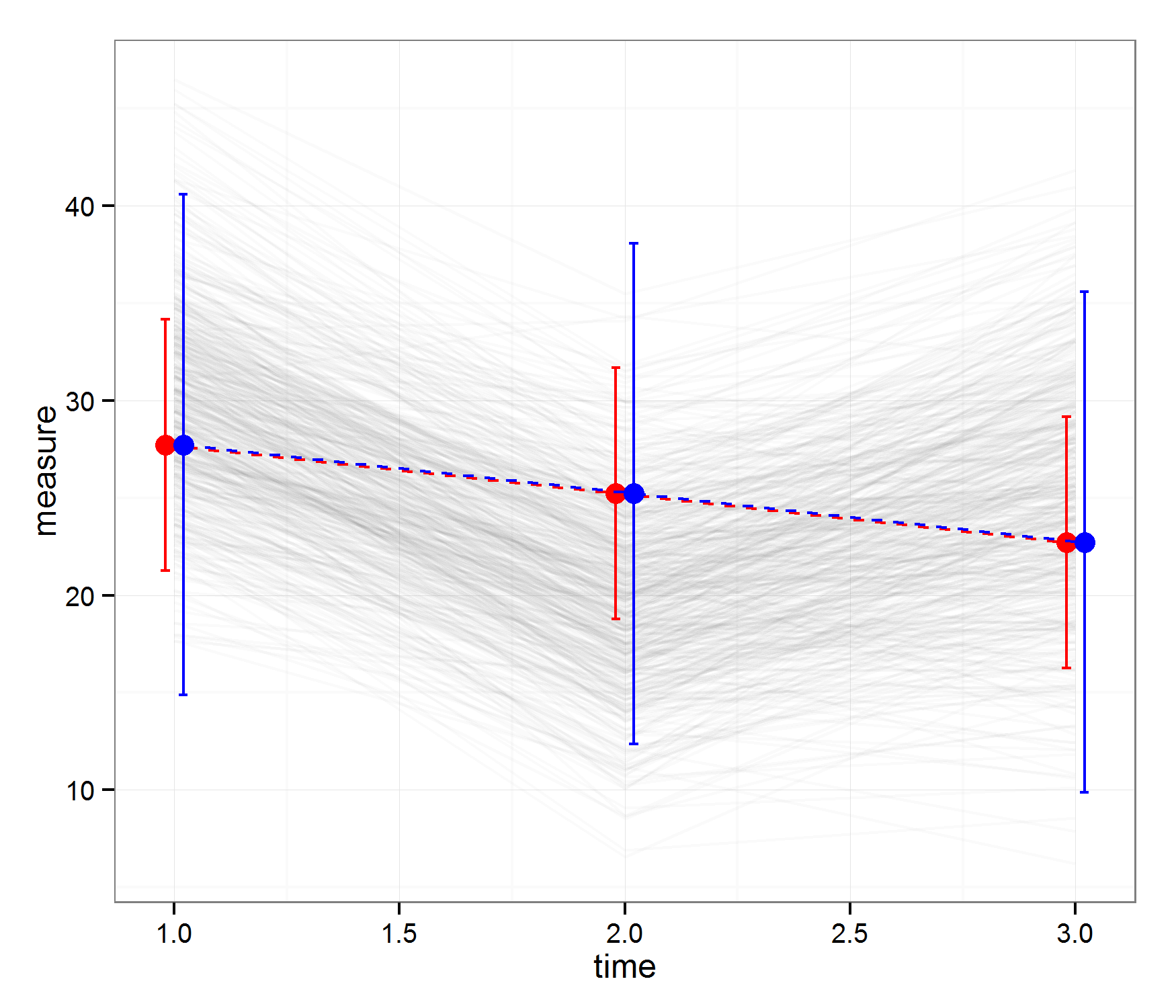
If you’re as data-sensitive as me, you should have probably noticed the fitted values aren’t quite fit to the actual data. This happens because the model is not specified well. Thereare at least two ways to specify the models better which we’ll talk about in upcoming posts. Stay tuned.