In the previous part of this tutorial, we build several models based on logistic regression. One aspect to be further considered is the decision threshold tuning that may help in reaching a better accuracy. We are going to show a procedure able to determine an optimal value for such purpose. ROC plots will be introduced as well.
Decision Threshold Tuning
As default, caret uses 0.5 as threshold decision value to be used as probability cutoff value. We are going to show how to tune such decision threshold to achieve a better training set accuracy. We then compare how the testing set accuracy changes accordingly.
Tuning Analysis
We load previously saved training, testing datasets together with the models we have already determined.
suppressPackageStartupMessages(library(caret))
suppressPackageStartupMessages(library(ROCR))
set.seed(1023)
readRDS(file="wf_log_reg_part2.rds")
The following tuning procedure explores a pool of cutoff values giving back a table reporting {cutoff, accuracy, specificity} triplets. Its inspection allows to identify the cutoff value providing with the highest accuracy. In case of a tie in accuracy value, we choose the lowest cutoff value of such.
glm.tune <- function(glm_model, dataset) {
   results <- data.frame()
   for (q in seq(0.2, 0.8, by = 0.02)) {
      fitted_values <- glm_model$finalModel$fitted.values
      prediction <- as.factor(ifelse(fitted_values >= q, "Yes", "No"))
      cm <- confusionMatrix(prediction, dataset$RainTomorrow)
      accuracy <- cm$overall["Accuracy"]
      specificity <- cm$byClass["Specificity"]
      results <- rbind(results, data.frame(cutoff=q, accuracy=accuracy, specificity = specificity))
   }
   rownames(results) <- NULL
   results
}
In the utility function above, we included also the specificity metrics. Specificity is defined as TN/(TN+FP) and in the next part of this series we will discuss some aspects of. Let us show an example of confusion matrix with some metrics computation to clarify the terminology.
    Reference
Prediction  No Yes
       No  203  42
       Yes   0   3

               Accuracy : 0.8306   = (TP+TN)/(TP+TN+FP+FN) = (203+3)/(203+3+42+0)
            Sensitivity : 1.00000  = TP/(TP+FN) = 203/(203+0)
            Specificity : 0.06667  = TN/(TN+FP) = 3/(3+42)
         Pos Pred Value : 0.82857  = TP/(TP+FP) = 203/(203+42)
         Neg Pred Value : 1.00000  = TN/(TN+FN) = 3/(3+0)
Please note that the “No” column is associated to a positive outcome, whilst “Yes” to a negative one. Specificity measure how good we are in predict that {RainTomorrow = “No”} and actually it is and this is something that we are going to investigate in next post of this series.
The logistic regression models to be tuned are:
mod9am_c1_fit: RainTomorrow ~ Cloud9am + Humidity9am + Pressure9am + Temp9am
mod3pm_c1_fit: RainTomorrow ~ Cloud3pm + Humidity3pm + Pressure3pm + Temp3pm
mod_ev_c2_fit: RainTomorrow ~ Cloud3pm + Humidity3pm + Pressure3pm + Temp3pm + WindGustDir
mod_ev_c3_fit: RainTomorrow ~ Pressure3pm + Sunshine
In the following analysis, for all models we determine the cutoff value providing with the highest accuracy.
glm.tune(mod9am_c1_fit, training)
   cutoff  accuracy specificity
1    0.20 0.7822581  0.73333333
2    0.22 0.7862903  0.71111111
3    0.24 0.7943548  0.68888889
4    0.26 0.8064516  0.64444444
5    0.28 0.8104839  0.64444444
6    0.30 0.8145161  0.60000000
7    0.32 0.8185484  0.57777778
8    0.34 0.8185484  0.51111111
9    0.36 0.8104839  0.46666667
10   0.38 0.8266129  0.46666667
11   0.40 0.8266129  0.40000000
12   0.42 0.8306452  0.40000000
13   0.44 0.8266129  0.37777778
14   0.46 0.8346774  0.35555556
15   0.48 0.8467742  0.33333333
16   0.50 0.8508065  0.31111111
17   0.52 0.8427419  0.26666667
18   0.54 0.8467742  0.26666667
19   0.56 0.8346774  0.20000000
20   0.58 0.8387097  0.20000000
21   0.60 0.8387097  0.20000000
22   0.62 0.8346774  0.17777778
23   0.64 0.8387097  0.17777778
24   0.66 0.8346774  0.15555556
25   0.68 0.8387097  0.15555556
26   0.70 0.8387097  0.13333333
27   0.72 0.8387097  0.13333333
28   0.74 0.8346774  0.11111111
29   0.76 0.8266129  0.06666667
30   0.78 0.8266129  0.06666667
31   0.80 0.8306452  0.06666667
The optimal cutoff value is equal to 0.5. In this case, we find the same cutoff value as the default the caret package takes advantage of for logistic regression models.
opt_cutoff <- 0.5
pred_test <- predict(mod9am_c1_fit, testing, type = "prob")
prediction = as.factor(ifelse(pred_test$Yes >= opt_cutoff, "Yes", "No"))
confusionMatrix(prediction, testing$RainTomorrow)
Confusion Matrix and Statistics

          Reference
Prediction No Yes
       No  80  12
       Yes  6   7

               Accuracy : 0.8286
                 95% CI : (0.7427, 0.8951)
    No Information Rate : 0.819
    P-Value [Acc > NIR] : 0.4602

                  Kappa : 0.3405
 Mcnemar's Test P-Value : 0.2386

            Sensitivity : 0.9302
            Specificity : 0.3684
         Pos Pred Value : 0.8696
         Neg Pred Value : 0.5385
             Prevalence : 0.8190
         Detection Rate : 0.7619
   Detection Prevalence : 0.8762
      Balanced Accuracy : 0.6493

       'Positive' Class : No
Then, tuning the 3PM model.
glm.tune(mod3pm_c1_fit, training)
  cutoff  accuracy specificity
1    0.20 0.8064516   0.7777778
2    0.22 0.8185484   0.7555556
3    0.24 0.8225806   0.7333333
4    0.26 0.8306452   0.6888889
5    0.28 0.8467742   0.6666667
6    0.30 0.8467742   0.6444444
7    0.32 0.8427419   0.6222222
8    0.34 0.8669355   0.6222222
9    0.36 0.8709677   0.6222222
10   0.38 0.8629032   0.5777778
11   0.40 0.8669355   0.5777778
12   0.42 0.8669355   0.5555556
13   0.44 0.8548387   0.4666667
14   0.46 0.8548387   0.4444444
15   0.48 0.8588710   0.4444444
16   0.50 0.8669355   0.4444444
17   0.52 0.8629032   0.4222222
18   0.54 0.8669355   0.4222222
19   0.56 0.8669355   0.3777778
20   0.58 0.8669355   0.3777778
21   0.60 0.8588710   0.3333333
22   0.62 0.8548387   0.3111111
23   0.64 0.8508065   0.2888889
24   0.66 0.8467742   0.2666667
25   0.68 0.8387097   0.2222222
26   0.70 0.8387097   0.2222222
27   0.72 0.8346774   0.2000000
28   0.74 0.8387097   0.1777778
29   0.76 0.8346774   0.1555556
30   0.78 0.8346774   0.1555556
31   0.80 0.8306452   0.1111111
The optimal cutoff value is equal to 0.36.
opt_cutoff <- 0.36
pred_test <- predict(mod3pm_c1_fit, testing, type="prob")
prediction = as.factor(ifelse(pred_test$Yes >= opt_cutoff, "Yes", "No"))
confusionMatrix(prediction, testing$RainTomorrow)
Confusion Matrix and Statistics

          Reference
Prediction No Yes
       No  81   5
       Yes  5  14

               Accuracy : 0.9048
                 95% CI : (0.8318, 0.9534)
    No Information Rate : 0.819
    P-Value [Acc > NIR] : 0.0112

                  Kappa : 0.6787
 Mcnemar's Test P-Value : 1.0000

            Sensitivity : 0.9419
            Specificity : 0.7368
         Pos Pred Value : 0.9419
         Neg Pred Value : 0.7368
             Prevalence : 0.8190
         Detection Rate : 0.7714
   Detection Prevalence : 0.8190
      Balanced Accuracy : 0.8394

       'Positive' Class : No
We improved the test accuracy, previously resulting as equal to 0.8857 and now equal to 0.9048 (please take a look at part #2 of this tutorial to know about the test accuracy with 0.5 cutoff value). Then, the first evening hours model.
glm.tune(mod_ev_c2_fit, training)
  cutoff  accuracy specificity
1    0.20 0.8387097   0.8444444
2    0.22 0.8467742   0.8222222
3    0.24 0.8548387   0.8222222
4    0.26 0.8629032   0.8000000
5    0.28 0.8588710   0.7333333
6    0.30 0.8709677   0.7333333
7    0.32 0.8790323   0.7111111
8    0.34 0.8830645   0.6888889
9    0.36 0.8870968   0.6666667
10   0.38 0.8870968   0.6666667
11   0.40 0.8951613   0.6666667
12   0.42 0.8991935   0.6666667
13   0.44 0.8991935   0.6666667
14   0.46 0.8951613   0.6444444
15   0.48 0.8951613   0.6222222
16   0.50 0.8951613   0.6222222
17   0.52 0.8951613   0.6000000
18   0.54 0.8911290   0.5777778
19   0.56 0.8911290   0.5777778
20   0.58 0.8951613   0.5777778
21   0.60 0.8911290   0.5555556
22   0.62 0.8870968   0.5111111
23   0.64 0.8830645   0.4888889
24   0.66 0.8830645   0.4666667
25   0.68 0.8790323   0.4222222
26   0.70 0.8709677   0.3555556
27   0.72 0.8548387   0.2666667
28   0.74 0.8508065   0.2444444
29   0.76 0.8427419   0.1777778
30   0.78 0.8387097   0.1555556
31   0.80 0.8387097   0.1555556
The optimal cutoff value is equal to 0.42.
opt_cutoff <- 0.42
pred_test <- predict(mod_ev_c2_fit, testing, type="prob")
prediction = as.factor(ifelse(pred_test$Yes >= opt_cutoff, "Yes", "No"))
confusionMatrix(prediction, testing$RainTomorrow)
Confusion Matrix and Statistics

          Reference
Prediction No Yes
       No  82   8
       Yes  4  11

               Accuracy : 0.8857
                 95% CI : (0.8089, 0.9395)
    No Information Rate : 0.819
    P-Value [Acc > NIR] : 0.04408

                  Kappa : 0.58
 Mcnemar's Test P-Value : 0.38648

            Sensitivity : 0.9535
            Specificity : 0.5789
         Pos Pred Value : 0.9111
         Neg Pred Value : 0.7333
             Prevalence : 0.8190
         Detection Rate : 0.7810
   Detection Prevalence : 0.8571
      Balanced Accuracy : 0.7662

       'Positive' Class : No
We did not improve the accuracy as the default cutoff value provides with the same. Other metrics changed and in particular we notice that the sensitivity decreased a little bit while the positive predicted value improved. Then the second evening hours model.
glm.tune(mod_ev_c3_fit, training)
 cutoff  accuracy specificity
1    0.20 0.8225806   0.8000000
2    0.22 0.8145161   0.7333333
3    0.24 0.8064516   0.6666667
4    0.26 0.8145161   0.6666667
5    0.28 0.8145161   0.6222222
6    0.30 0.8185484   0.6222222
7    0.32 0.8266129   0.6000000
8    0.34 0.8185484   0.5555556
9    0.36 0.8306452   0.5333333
10   0.38 0.8467742   0.5333333
11   0.40 0.8467742   0.5111111
12   0.42 0.8427419   0.4666667
13   0.44 0.8508065   0.4666667
14   0.46 0.8467742   0.4222222
15   0.48 0.8467742   0.4000000
16   0.50 0.8508065   0.4000000
17   0.52 0.8548387   0.4000000
18   0.54 0.8508065   0.3777778
19   0.56 0.8669355   0.3777778
20   0.58 0.8669355   0.3555556
21   0.60 0.8629032   0.3333333
22   0.62 0.8588710   0.3111111
23   0.64 0.8548387   0.2888889
24   0.66 0.8508065   0.2666667
25   0.68 0.8467742   0.2444444
26   0.70 0.8387097   0.2000000
27   0.72 0.8387097   0.1777778
28   0.74 0.8346774   0.1555556
29   0.76 0.8306452   0.1333333
30   0.78 0.8306452   0.1333333
31   0.80 0.8306452   0.1333333
The optimal cutoff value is equal to 0.56.
opt_cutoff <- 0.56
pred_test <- predict(mod_ev_c3_fit, testing, type="prob")
prediction = as.factor(ifelse(pred_test$Yes >= opt_cutoff, "Yes", "No")
confusionMatrix(prediction, testing$RainTomorrow)
Confusion Matrix and Statistics

          Reference
Prediction No Yes
       No  82   8
       Yes  4  11

               Accuracy : 0.8857
                 95% CI : (0.8089, 0.9395)
    No Information Rate : 0.819
    P-Value [Acc > NIR] : 0.04408

                  Kappa : 0.58
 Mcnemar's Test P-Value : 0.38648

            Sensitivity : 0.9535
            Specificity : 0.5789
         Pos Pred Value : 0.9111
         Neg Pred Value : 0.7333
             Prevalence : 0.8190
         Detection Rate : 0.7810
   Detection Prevalence : 0.8571
      Balanced Accuracy : 0.7662

       'Positive' Class : No
In this case, we did not improved the accuracy of this model. Other metrics changed and in particular we notice that the sensitivity is slightly higher than the default cutoff driven value (0.9419), and the positive predicted value decreased a little bit (for default cutoff was 0.9205).
ROC analysis
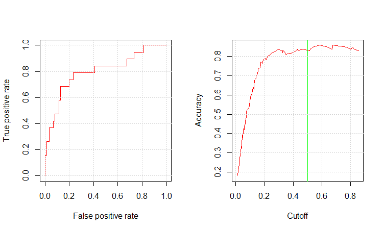
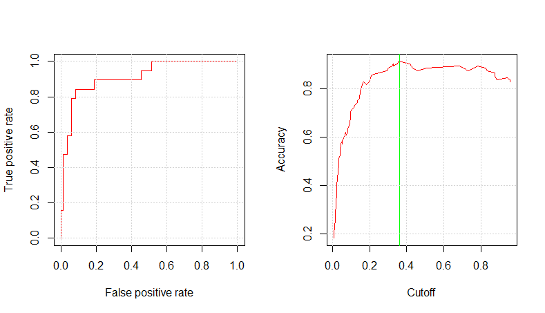
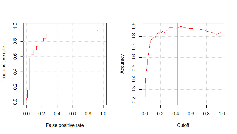
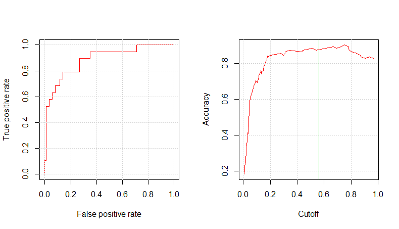
To have a visual understanding of the classification performances and compute further metrics, we are going to take advantage of the ROCr package facilities. We plot ROC curves and determine the corresponding AUC value. That is going to be done for each model. The function used to accomplish with this task is the following.
glm.perf.plot <- function (prediction, cutoff) {
    perf <- performance(prediction, measure = "tpr", x.measure = "fpr")
    par(mfrow=(c(1,2)))
    plot(perf, col="red")
    grid()
    perf <- performance(prediction, measure = "acc", x.measure = "cutoff")
    plot(perf, col="red")
    abline(v = cutoff, col="green")
    grid()
    auc_res <- performance(prediction, "auc")
    [email protected][[1]]
}
In the following, each model will be considered, AUC value printed out and ROC plots given.
mod9am_pred_prob <- predict(mod9am_c1_fit, testing, type="prob")
mod9am_pred_resp <- prediction(mod9am_pred_prob$Yes,  testing$RainTomorrow)
glm.perf.plot(mod9am_pred_resp, 0.5)
[1] 0.8004896
mod3pm_pred_prob <- predict(mod3pm_c1_fit, testing, type="prob")
mod3pm_pred_resp <- prediction(mod3pm_pred_prob$Yes,  testing$RainTomorrow)
glm.perf.plot(mod3pm_pred_resp, 0.36)
[1] 0.9155447
The 3PM model shows the highest AUC value among all the models.
mod_ev_c2_prob <- predict(mod_ev_c2_fit, testing, type="prob")
mod_ev_c2_pred_resp <- prediction(mod_ev_c2_prob$Yes
,  testing$RainTomorrow)
glm.perf.plot(mod_ev_c2_pred_resp, 0.42)
[1] 0.8390453
mod_ev_c3_prob <- predict(mod_ev_c3_fit, testing, type="prob")
mod_ev_c3_pred_resp <- prediction(mod_ev_c3_prob$Yes,  testing$RainTomorrow)
glm.perf.plot(mod_ev_c3_pred_resp, 0.56)
[1] 0.8886169
Conclusions
By tuning the decision threshold, we were able to improve training and testing set accuracy. It turned out the 3PM model achieved a satisfactory accuracy. ROC plots gave us an understanding of how true/false positive rates vary and what is the accuracy obtained by a specific decision threshold value (i.e. cutoff value). Ultimately, AUC values were reported.
If you have any questions, please feel free to comment below.


