Classification is a supervised machine learning technique in which the dataset which we are analyzing has some inputs Xi and a response variable Y which is a discrete valued variable.Discrete valued means the variable has a finite set of values.In more specific terms in classification the response variable has some categorical values.In R we call such values as factor variables. For example-Y∈ (Male,Female) or (0,1) or (High,low,medium) etc are the best examples of the response variable Y in a classification problem.
Now our task in a typical classification problem is to compute the mapping function(also called hypotheses) f : X–>Y which maps and relates inputs to target variable which it learns from the training data that we feed the learner.Now given some inputs the learning algorithm will learn from the data and will compute the probabilities of occurrence of each class label K where Y \in K.
Almost all the classifiers use a conditional probability model C(X) to compute the probabilities of the class labels.
C(X) = P(Y \in K | X) = \frac{P(X \cap Y)}{P(X)}
Definitely, there are a few exceptions which directly don’t use a conditional probability model(e.g-SVM) to classify data but in general, all classifiers use the conditional probability model.
Text Classification
Now in this article I am going to classify text messages as either Spam or Ham.As the dataset will have text messages which are unstructured in nature so we will require some basic natural language processing to compute word frequencies, tokenizing texts, and calculating document-feature matrix etc.
The dataset is taken from Kaggle’s SMS Spam Collection Spam Dataset.
Implementation in R
We will use a very nice package called quanteda which is used for managing, processing and analyzing text data.I urge the readers to go and read the documentation for the package and how it works.
Requiring the necessary packages–
require(quanteda)#natural language processing package
?quanteda
require(RColorBrewer)
require(ggplot2)
Copy
Let’s load the dataset.
spam=read.csv("../Datasets/spam.csv",header=TRUE, sep=",", quote='\"\"', stringsAsFactors=FALSE)

table(spam$v1)
##
##  ham spam
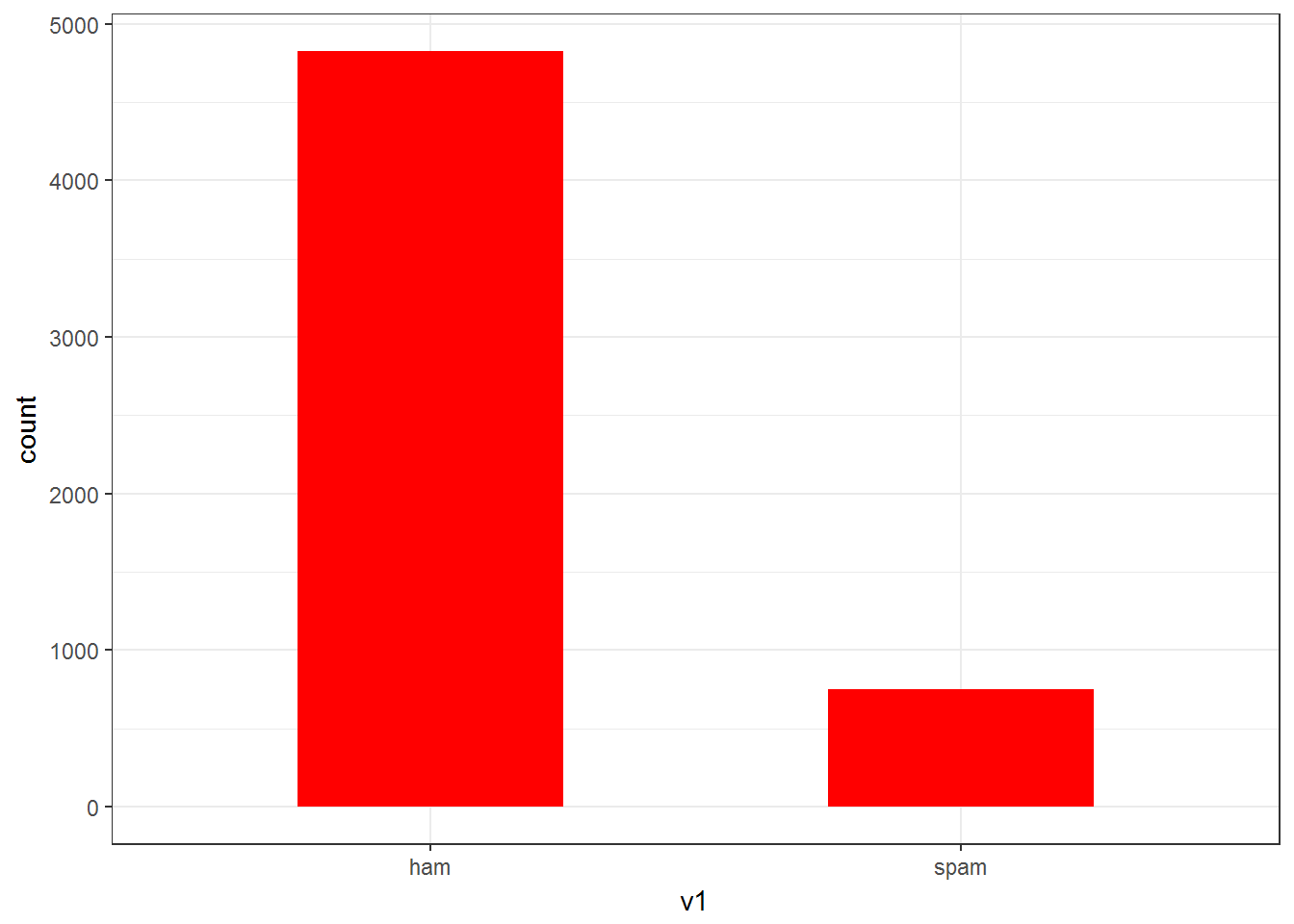
## 4825  747

Copy
As we can observe there are more number of ham messages than spam.
let’s plot a barplot-

Now let’s add appropriate names to the columns.
names(spam)<-c("type","message")
head(spam)
##   type
## 1  ham
## 2  ham
## 3 spam
## 4  ham
## 5  ham
## 6 spam
##                                                                                                                                                       message
## 1                                             Go until jurong point, crazy.. Available only in bugis n great world la e buffet... Cine there got amore wat...
## 2                                                                                                                               Ok lar... Joking wif u oni...
## 3 Free entry in 2 a wkly comp to win FA Cup final tkts 21st May 2005. Text FA to 87121 to receive entry question(std txt rate)T&C's apply 08452810075over18's
## 4                                                                                                           U dun say so early hor... U c already then say...
## 5                                                                                               Nah I don't think he goes to usf, he lives around here though
## 6        FreeMsg Hey there darling it's been 3 week's now and no word back! I'd like some fun you up for it still? Tb ok! XxX std chgs to send, å£1.50 to rcv
##   NA NA NA
## 1
## 2
## 3
## 4
## 5
## 6

Copy
Next thing we need to do is a random sampling of data i.e shuffling it.We can randomize our data using the sample() command.If the data is not stored in a random distribution, this will help to ensure that we are dealing with a random draw from our data. The set.seed() is to ensure reproducible results.
set.seed(2012)
spam<-spam[sample(nrow(spam)),] #randomly shuffling the dataset
Copy
Building the Wordclouds
Firstly, I will use quanteda’s corpus() command to construct a corpus from the text field of our raw data.A corpus can be thought of as a master copy of our dataset from which we can pull subsets or observations as needed.
After this I will attach the label field as a document variable to the corpus using the docvars() command. We attach label as a variable directly to our corpus so that we can associate SMS messages with their respective ham/spam label later in the analysis.
?corpus #to search more on this method
msg.corpus<-corpus(spam$message)

docvars(msg.corpus)<-spam$type   #attaching the class labels to the corpus message text


Copy
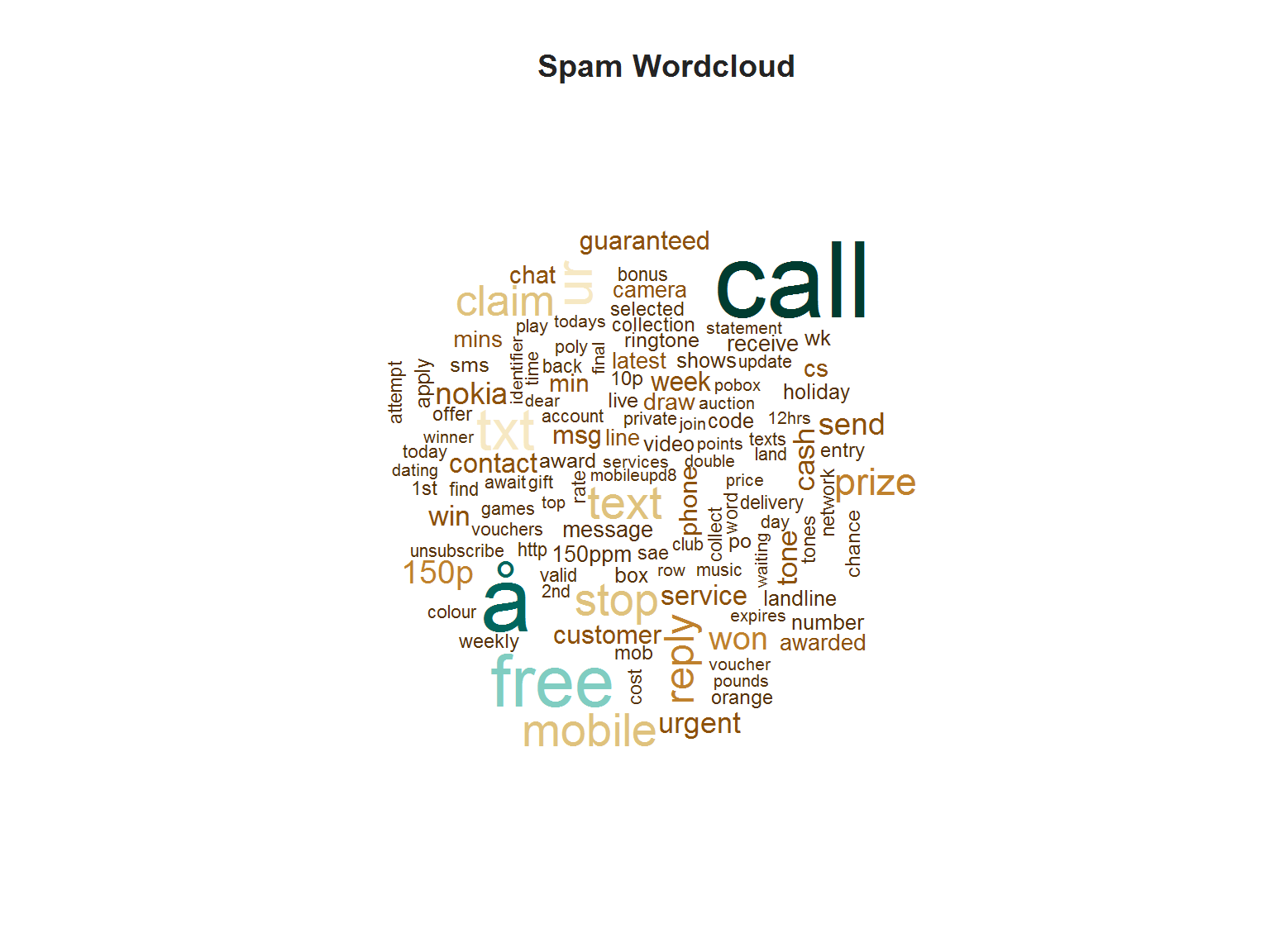
Let’s plot the word-cloud now-
First, we will subset and filter all the spam text messages from the message corpus.Then we will generate a document feature matrix which is a sparse matrix consisting of the frequency of words that occur in a document.The rows represent the document and column represent the words/terms of the sentence which show which documents contain which terms and how many times they appear.
#subsetting only the spam messages
spam.plot<-corpus_subset(msg.corpus,docvar1=="spam")

#now creating a document-feature matrix using dfm()
spam.plot<-dfm(spam.plot, tolower = TRUE, remove_punct = TRUE, remove_twitter = TRUE, remove_numbers = TRUE, remove=stopwords("SMART"))

spam.col <- brewer.pal(10, "BrBG")

textplot_wordcloud(spam.plot, min.freq = 16, color = spam.col)
title("Spam Wordcloud", col.main = "grey14")
Copy
Word cloud for Spam messages–
The above plot is a wordcloud which is an amazing way of visualizing and understanding textual data and visually represent the contents in sentences.What is does is it picks and selects the most commonly occurring words in the sentences i.e the words having the highest frequencies and plots them, the more the frequency of a particular word the greater is the size of the word in the word-cloud.
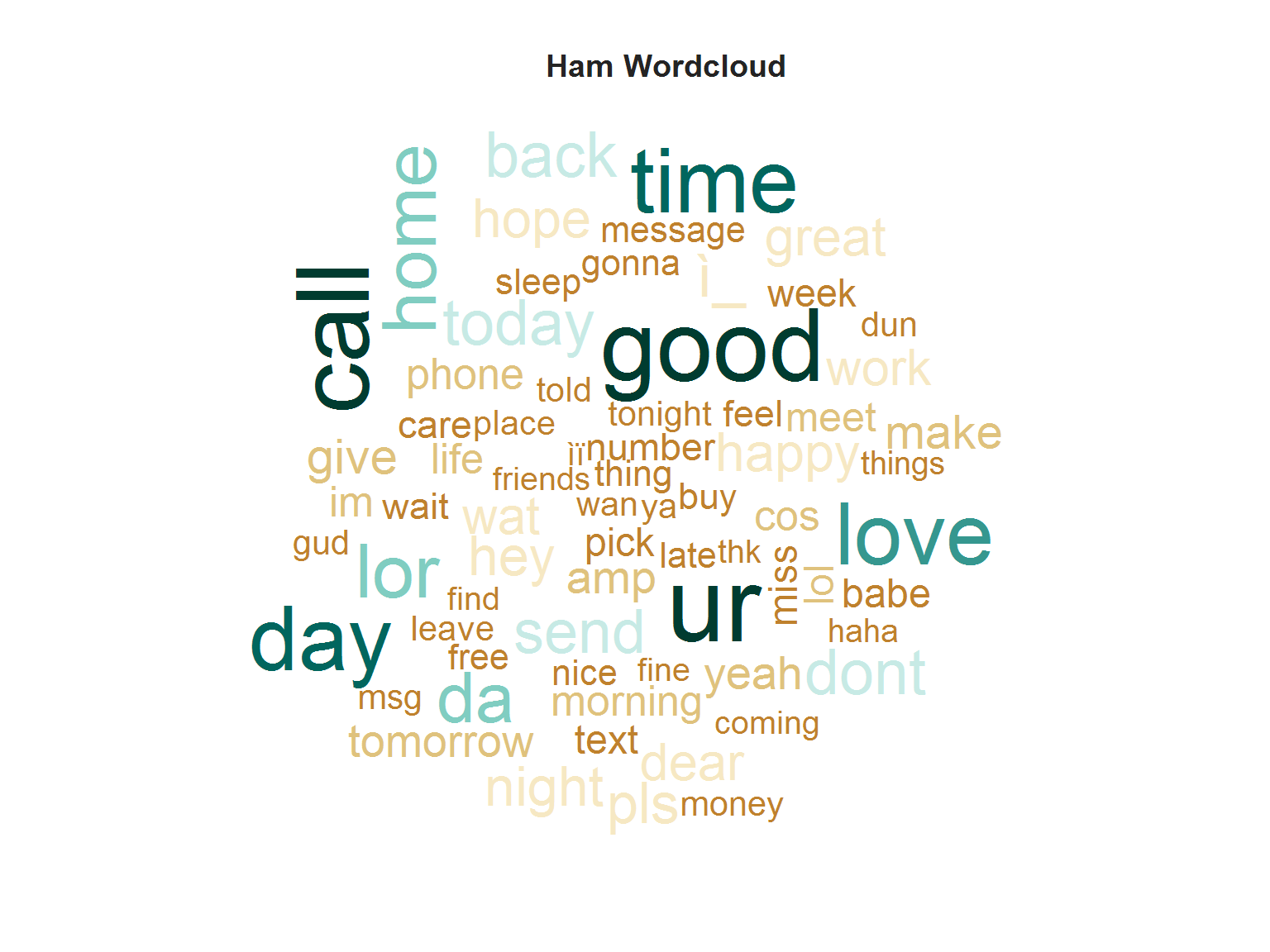
Generating the Ham wordcloud
We will use the same procedure like we used in generating the spam wordcloud.
ham.plot<-corpus_subset(msg.corpus,docvar1=="ham")
ham.plot<-dfm(ham.plot,tolower = TRUE, remove_punct = TRUE, remove_twitter = TRUE, remove_numbers = TRUE,remove=c("gt", "lt", stopwords("SMART")))
ham.col=brewer.pal(10, "BrBG")
textplot_wordcloud(ham.plot,min.freq=50,colors=ham.col,fixed.asp=TRUE)
title("Ham Wordcloud",col.main = "grey14")
Copy
The above-plotted word-clouds are an amazing tool for knowing what are the most frequently occurring words that appear in Spam and Ham messages.
Predictive Modelling
Now let’s train a Naive Bayes text classifier to compute the probabilities of a message being (spam,ham) i.e P(Y=Spam | message) and P(Y=ham | message) .
Naive Bayes classifiers are a class of simple linear classifiers which use conditional probability models based on Bayes Theoram i.e
C(X)=P(Y=K_j | X_i)=P(X_1|Y).P(X_2|Y)…P(X_i|Y)P(Y=K_j)
Where X_i are the number of inputs and Y is a categorical response variable and K_j are the number of class labels.
The special thing about Naive Bayes classifiers is that they follow Conditional Independence Theoram i.e they assume that the features X_i are uncorrelated and independent of each other which is often a crude and impractical assumption,but still they are nice and simple classifiers which perform well most of the times too, because we are only concerned with the probability values.Secondly, they assume that the data samples are drawn from an identical and independent distribution- IID is the term which is famous in Statistics.
Let’s separate the training and test data-
#separating Train and test data
spam.train<-spam[1:4458,]
spam.test<-spam[4458:nrow(spam),]

msg.dfm <- dfm(msg.corpus, tolower = TRUE)  #generating document freq matrix
msg.dfm <- dfm_trim(msg.dfm, min_count = 5, min_docfreq = 3)
msg.dfm <- dfm_weight(msg.dfm, type = "tfidf")

head(msg.dfm)

#trining and testing data of dfm
msg.dfm.train<-msg.dfm[1:4458,]

msg.dfm.test<-msg.dfm[4458:nrow(spam),]

 > #head(msg.dfm)
Document-feature matrix of: 5,572 documents, 1,932 features (99.3% sparse).
(showing first 6 documents and first 6 features)
       features
docs     nothing     much        ,       at     home         .
  text1 2.166228 1.712587 0.644264 1.170823 1.539185 0.1999622
  text2 0.000000 0.000000 0.000000 0.000000 0.000000 0.1999622
  text3 0.000000 0.000000 0.000000 0.000000 1.539185 0.1999622
  text4 0.000000 0.000000 0.000000 0.000000 0.000000 0.0000000
  text5 0.000000 0.000000 0.000000 0.000000 0.000000 1.7996602
  text6 0.000000 0.000000 0.644264 0.000000 0.000000 0.1999622

Copy
Please read the documentation of the above functions used for processing the document-feature-matrix to know more about the functions and their major use.
Training the Naive Bayes classifier-
nb.classifier<-textmodel_NB(msg.dfm.train,spam.train[,1])
nb.classifier
## Fitted Naive Bayes model:
## Call:
##  textmodel_NB.dfm(x = msg.dfm.train, y = spam.train[, 1])
##
##
## Training classes and priors:
## spam  ham
##  0.5  0.5
##
##        Likelihoods:      Class Posteriors:
## 30 x 4 Matrix of class "dgeMatrix"
##                 spam          ham       spam       ham
## you     5.001507e-03 0.0096798156 0.34067144 0.6593286
## have    4.322289e-03 0.0042303673 0.50537386 0.4946261
## 1       2.695748e-03 0.0009529526 0.73882413 0.2611759
## new     3.492485e-03 0.0010753934 0.76457487 0.2354251
## .       6.965338e-03 0.0168302131 0.29271598 0.7072840
## please  2.339097e-03 0.0011593603 0.66860811 0.3313919
## call    1.058603e-02 0.0021859571 0.82884759 0.1711524
## i       8.439760e-04 0.0112106647 0.07001254 0.9299875
## wait    1.860817e-04 0.0011538316 0.13887596 0.8611240
## for     5.699340e-03 0.0045025239 0.55865674 0.4413433
## hope    2.334040e-04 0.0017258550 0.11912872 0.8808713
## tonight 1.137075e-04 0.0011106417 0.09287182 0.9071282
## too     3.802754e-05 0.0017024748 0.02184860 0.9781514
## bad     1.232420e-04 0.0006045270 0.16934219 0.8306578
## as      1.339518e-03 0.0020699791 0.39287852 0.6071215
## well    2.938089e-04 0.0017334850 0.14492664 0.8550734
## but     2.528948e-04 0.0043933716 0.05442968 0.9455703
## rock    3.802754e-05 0.0002684845 0.12406542 0.8759346
## night   3.003905e-04 0.0017976398 0.14317739 0.8568226
## anyway  3.802754e-05 0.0005405216 0.06572915 0.9342709
## going   1.538819e-04 0.0023951976 0.06036762 0.9396324
## a       7.856726e-03 0.0064918622 0.54756091 0.4524391
## now     6.254232e-03 0.0028758075 0.68501697 0.3149830
## good    6.723203e-04 0.0030342352 0.18138681 0.8186132
## speak   8.003838e-04 0.0004728416 0.62862694 0.3713731
## to      1.113210e-02 0.0075761991 0.59503541 0.4049646
## soon    2.642059e-04 0.0010608467 0.19939274 0.8006073
## today   1.120666e-03 0.0019041688 0.37048833 0.6295117
## is      4.451802e-03 0.0058153446 0.43359683 0.5664032
## accept  3.802754e-05 0.0003188419 0.10655871 0.8934413


Copy
The model outputs the Probabilities of the message being Spam or ham.
Let’s Test the Model
pred<-predict(nb.classifier,msg.dfm.test)

#generating a confusion matrix

# use pred$nb.predicted to extract the class labels
table(predicted=pred$nb.predicted,actual=spam.test[,1])
##       actual
## predicted ham spam
##      ham  952    7
##      spam  16  140

Copy
16 text examples wrongly classified for ham and 7 examples wrongly classified for spam.
In the Confusion matrix,the diagonals are the correctly classified examples and the off-diagonals are the incorrectly classified text instances.
Now let’s calculate the accuracy of the model –
#acccuracy of the classifier on Test data
mean(pred$nb.predicted==spam.test[,1])*100
## [1] 97.93722

Copy
Now 98% accuracy is a good amount of accuracy on unseen random test data.
Conclusion
This was a simple article on classifying text messages as ham or spam using some basic natural language processing and then building a naive Bayes text classifier.I urge the readers to implement and use the knowledge acquired from this article in making their own text classifiers and solving different problems related to text processing and NLP etc.
Ofcourse, there are various other packages to do text processing and building such models.
Hope you guys liked the article, make sure to like and share it.

