The present tutorial analyses the Tennis Grand Slam tournaments main results from the statistical point of view. Specifically, I try to answer the following questions:
– How to fit the distribution of the Grand Slam tournaments number of victories across players?
– How to compute the probability of having player’s victories greater than a specific number?
– How the number of Grand Slam tournaments winners increases along with time?
– How can we assign a metric to the tennis players based on the number of Grand Slam tournaments they won?
Our dataset is provided within ref. [1], whose content is based on what reported by the ESP site at: ESPN site tennis history table.
Packages
suppressPackageStartupMessages(library(fitdistrplus))
suppressPackageStartupMessages(library(extremevalues))
suppressPackageStartupMessages(library(dplyr))
suppressPackageStartupMessages(library(knitr))
suppressPackageStartupMessages(library(ggplot2))
Analysis
The analysis within the present tutorial is organized as follows:
- a basic data exploration is run
- log-normal distribution is fit against the Grand Slam tournaments victories data
- regression analysis is presented in order to evaluate the increase of tennis Grand Slam champions along with time
- population statistical dispersion is evaluated to determine a Tennis Quotient assigned to tournaments’ winners
Basic Data Exploration
Loading the Tennis Grand Slam tournaments dataset and running a basic data exploration.
url_file <- "https://datascienceplus.com/wp-content/uploads/2017/12/tennis-grand-slam-winners_end2017.txt"
slam_win <- read.delim(url(url_file), sep="\t", stringsAsFactors = FALSE)
dim(slam_win)
[1] 489   4
kable(head(slam_win), row.names=FALSE)
| YEAR|TOURNAMENT      |WINNER        |RUNNER.UP      |
|----:|:---------------|:-------------|:--------------|
| 2017|U.S. Open       |Rafael Nadal  |Kevin Anderson |
| 2017|Wimbledon       |Roger Federer |Marin Cilic    |
| 2017|French Open     |Rafael Nadal  |Stan Wavrinka  |
| 2017|Australian Open |Roger Federer |Rafael Nadal   |
| 2016|U.S. Open       |Stan Wawrinka |Novak Djokovic |
| 2016|Wimbledon       |Andy Murray   |Milos Raonic   |
kable(tail(slam_win), row.names=FALSE)
| YEAR|TOURNAMENT |WINNER           |RUNNER.UP          |
|----:|:----------|:----------------|:------------------|
| 1881|U.S. Open  |Richard D. Sears |William E. Glyn    |
| 1881|Wimbledon  |William Renshaw  |John Hartley       |
| 1880|Wimbledon  |John Hartley     |Herbert Lawford    |
| 1879|Wimbledon  |John Hartley     |V. St. Leger Gould |
| 1878|Wimbledon  |Frank Hadow      |Spencer Gore       |
| 1877|Wimbledon  |Spencer Gore     |William Marshall   |
nr <- nrow(slam_win)
start_year <- slam_win[nr, "YEAR"]
end_year <- slam_win[1, "YEAR"]
(years_span <- end_year - start_year + 1)
[1] 141
(total_slam_winners <- length(unique(slam_win[,"WINNER"])))
[1] 166
So we have 166 winners spanning over 141 years of Tennis Grand Slam tournaments. We observe that during first and second World Wars, a reduced number of Grand Slam tournaments were played for obvious reasons.
slam_win_df <- as.data.frame(table(slam_win[,"WINNER"]))
slam_win_df =  slam_win_df %>% arrange(desc(Freq))
# computing champions' leaderboard position
pos <- rep(0, nrow(slam_win_df))
pos[1] <- 1
for(i in 2:nrow(slam_win_df)) {
  pos[i] <- ifelse(slam_win_df$Freq[i] != slam_win_df$Freq[i-1], i, pos[i-1])
}
last_win_year = sapply(slam_win_df$Var1, function(x) {slam_win %>% filter(WINNER == x) %>% dplyr::select(YEAR) %>% max()})
# creating and showing leaderboard dataframe
slam_winners <- data.frame(RANK = pos,
                           PLAYER = slam_win_df$Var1,
                           WINS = slam_win_df$Freq,
                           LAST_WIN_YEAR = last_win_year)
kable(slam_winners)
| RANK|PLAYER                      | WINS| LAST_WIN_YEAR|
|----:|:---------------------------|----:|-------------:|
|    1|Roger Federer               |   19|          2017|
|    2|Rafael Nadal                |   16|          2017|
|    3|Pete Sampras                |   14|          2002|
|    4|Novak Djokovic              |   12|          2016|
|    4|Roy Emerson                 |   12|          1967|
...
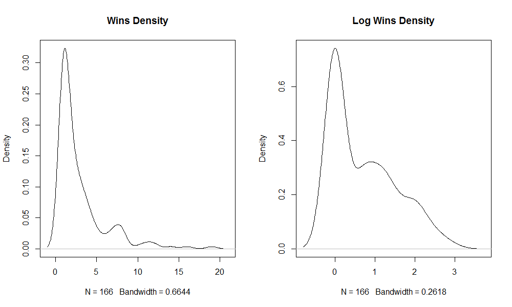
The WINS and log(WINS) distribution density are shown.
par(mfrow=c(1,2))
plot(density(slam_winners$WINS), main = "Wins Density")
plot(density(log(slam_winners$WINS)), main = "Log Wins Density")
Gives this plot:
You may want to arrange the same dataframe ordering by the champions’ last win year.
par(mfrow=c(1,1))
slam_winners_last_win_year = slam_winners %>% arrange(LAST_WIN_YEAR)
kable(slam_winners %>% arrange(desc(LAST_WIN_YEAR)))
| RANK|PLAYER                      | WINS| LAST_WIN_YEAR|
|----:|:---------------------------|----:|-------------:|
|    1|Roger Federer               |   19|          2017|
|    2|Rafael Nadal                |   16|          2017|
|    4|Novak Djokovic              |   12|          2016|
|   43|Andy Murray                 |    3|          2016|
...
We may want to visualize the timeline of the number of Tennis Grand Slam champions.
df_nwin = data.frame()
for (year in start_year : end_year) {
  n_slam_winners = slam_win %>% filter(YEAR <= year) %>% dplyr::select(WINNER) %>% unique %>% nrow
  df_nwin = rbind(df_nwin, data.frame(YEAR = year, N_WINNERS = n_slam_winners))
}
plot(x = df_nwin$YEAR, y = df_nwin$N_WINNERS, type ='s', xlab = "year", ylab = "no_winners")
grid()
Gives this plot:

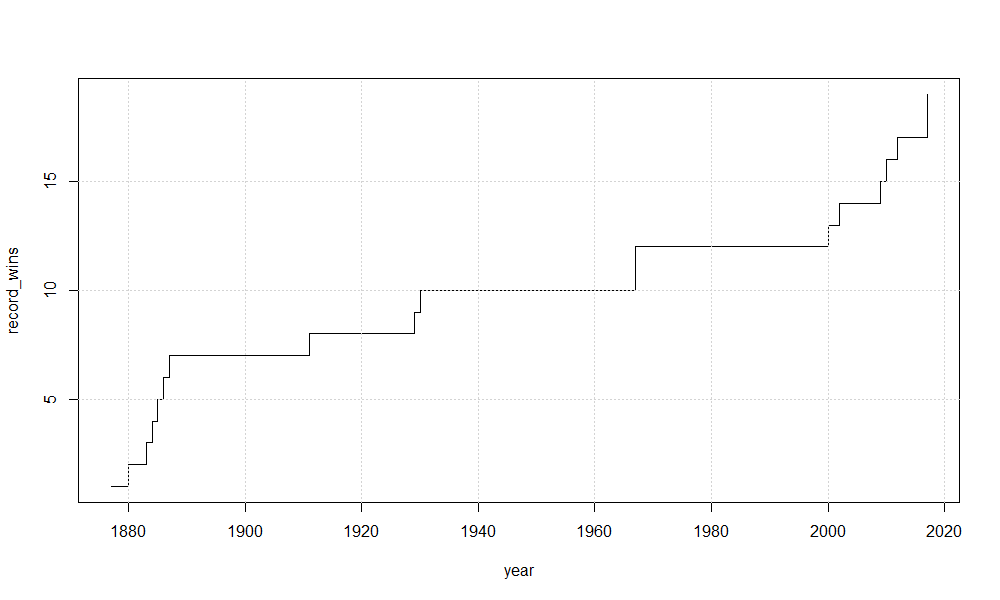
We may want to visualize the timeline of the Grand Slam tournaments wins record.
df2_nwin = data.frame()
for (year in start_year : end_year) {
  slam_win_years = slam_win %>% filter(YEAR <= year)
  slam_win_record = as.data.frame(table(slam_win_years[,"WINNER"]))
  df2_nwin = rbind(df2_nwin, data.frame(YEAR = year, RECORD_WINS = max(slam_win_record$Freq)))
}
plot(x = df2_nwin$YEAR, y = df2_nwin$RECORD_WINS, type ='s', xlab = "year", ylab = "record_wins")
grid()
Gives this plot:
It is interesting to have a look at the number of wins frequency.
wins_frequency <- as.data.frame(table(slam_winners[,"WINS"]))
colnames(wins_frequency) <- c("WINS", "FREQUENCY")
kable(wins_frequency)
|WINS | FREQUENCY|
|:----|---------:|
|1    |        80|
|2    |        25|
|3    |        19|
|4    |        12|
|5    |         5|
|6    |         3|
|7    |         6|
|8    |         8|
|10   |         1|
|11   |         2|
|12   |         2|
|14   |         1|
|16   |         1|
|19   |         1|
summary(slam_winners[,"WINS"])
Min. 1st Qu.  Median    Mean 3rd Qu.    Max.
  1.000   1.000   2.000   2.946   3.750  19.000
Probabilistic Distribution Fit
We now take advantage of the fitdist() function within the fitdistr package to fit a lognormal distribution for our Grand Slam wins data.
fw <- fitdist(slam_winners$WINS, "lnorm")
summary(fw)
Fitting of the distribution ' lnorm ' by maximum likelihood
Parameters :
         estimate Std. Error
meanlog 0.7047927 0.06257959
sdlog   0.8062817 0.04425015
Loglikelihood:  -316.7959   AIC:  637.5918   BIC:  643.8158
Correlation matrix:
        meanlog sdlog
meanlog       1     0
sdlog         0     1
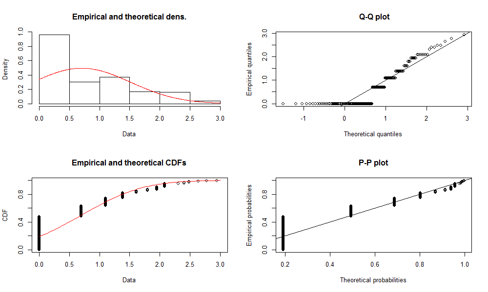
Then we can plot the distribution fit results.
plot(fw)
Gives this plot:

# left outliers quantile
left_thresh <- 0.05
# right outliers quantile
right_thresh <- 0.95
# determining the outliers
slam_outlier <- getOutliersI(as.vector(slam_winners$WINS),
FLim = c(left_thresh, right_thresh),
distribution = "lognormal")
# outliers are plotted in red color
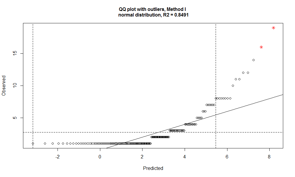
outlierPlot(slam_winners$WINS, slam_outlier, mode="qq")
Gives this plot:
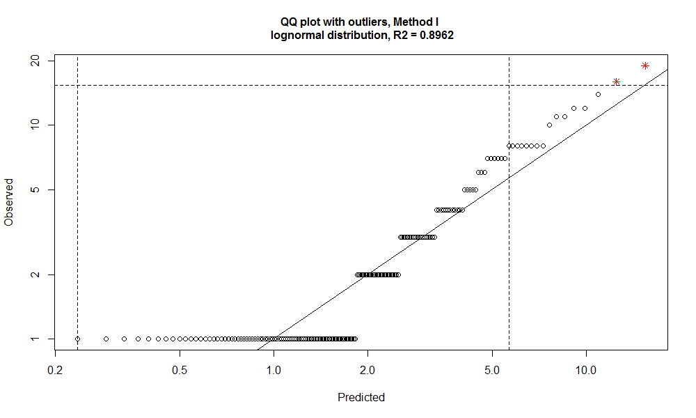
The outliers are:
slam_winners[slam_outlier$iRight,]
 RANK        PLAYER WINS LAST_WIN_YEAR
1    1 Roger Federer   19          2017
2    2  Rafael Nadal   16          2017
The mean and standard deviation associated to the log-normal fit are:
(mean_log <- fw$estimate["meanlog"])
meanlog
0.7047927
(sd_log <- fw$estimate["sdlog"])
sdlog
0.8062817
Now we compute the probability associated with 19 and 16 wins.
# clearing names
names(mean_log) <- NULL
names(sd_log) <- NULL
# probability associated to 19 wins performance or more
(lnorm_19 <- plnorm(19, mean_log, sd_log, lower.tail=FALSE))
[1] 0.002736863
# probability associated to 16 wins performance or more
(lnorm_16 <- plnorm(16, mean_log, sd_log, lower.tail=FALSE))
[1] 0.005164628
However, if a random variable follows a log-normal distribution, its logarithm follows a normal distribution. Hence we fit the logarithm of the variable under analysis using a normal distribution and compare the results with above log-normal fit.
fw_norm <- fitdist(log(slam_winners$WINS), "norm")
summary(fw_norm)
Fitting of the distribution ' norm ' by maximum likelihood
Parameters :
      estimate Std. Error
mean 0.7047927 0.06257959
sd   0.8062817 0.04425015
Loglikelihood:  -199.8003   AIC:  403.6006   BIC:  409.8246
Correlation matrix:
     mean sd
mean    1  0
sd      0  1
Similarly, we plot the fit results.
plot(fw_norm)
Gives this plot:
# left outliers quantile
left_thresh <- 0.05
# right outliers quantile
right_thresh <- 0.95
slam_outlier <- getOutliersI(log(as.vector(slam_winners$WINS)),
                             FLim = c(left_thresh, right_thresh),
                             distribution = "normal")
outlierPlot(slam_winners$WINS, slam_outlier, mode="qq")
Gives this plot:
The outliers are:
slam_winners[slam_outlier$iRight,]
 RANK        PLAYER WINS LAST_WIN_YEAR
1    1 Roger Federer   19          2017
2    2  Rafael Nadal   16          2017
The mean and standard deviation values are:
# mean and standard deviation of the fitted lognormal distribution
(mean_norm <- fw_norm$estimate["mean"])
mean
0.7047927
(sd_norm <- fw_norm$estimate["sd"])
 sd
0.8062817
As we can see above, same fitting parameters result from the two approaches, even though with different log-likelihood, AIC and BIC metrics. Now we compute the probability associated to 19 and 16 wins together with their distance from the mean in terms of multiples of the standard deviation.
# clearing names
names(mean_norm) <- NULL
names(sd_norm) <- NULL
# probability associated to the 19 wins performance or better
(norm_19 <- pnorm(log(19), mean_norm, sd_norm, lower.tail=FALSE))
[1] 0.002736863
# standard deviation times from the mean associated to 19 wins
(deviation_19 <- (log(19) - mean_norm)/sd_norm)

[1] 2.777747
# probability associated to the 16 wins performance or better
(norm_16 <- pnorm(log(16), mean_norm, sd_norm, lower.tail=FALSE))

[1] 0.005164628
# standard deviation times from the mean associated to 16 wins
(deviation_16 <- (log(16) - mean_norm)/sd_norm)

[1] 2.564608
As we can see above, we also obtained the same probability value as resulting from the log-normal distribution fit. In the following, we consider the second fitting approach (the one which takes the log of the original variable) for easing the computation of the distance from the mean in terms of multiples of the standard deviation.
Regression Analysis
Let us see again the plot of the number of tennis Grand Slam winners against their timeline.
year <- df_nwin $YEAR
winners <- df_nwin$N_WINNERS
plot(x = year, y = winners, type ='l')
grid()
Gives this plot:
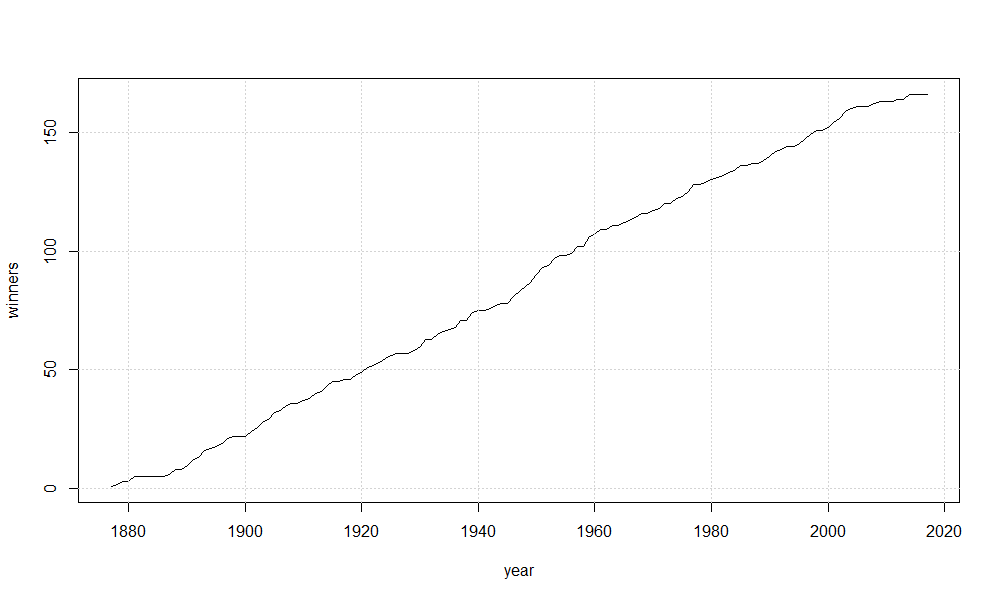
It is visually evident the linear relationship between the variables. Hence, a linear regression would help in understanding how many newbie Grand Slam winners we may have each year.
year_lm <- lm(winners ~ year)
summary(year_lm)
Call:
lm(formula = winners ~ year)

Residuals:
    Min      1Q  Median      3Q     Max
-9.8506 -1.9810 -0.4683  2.6102  6.2866

Coefficients:
              Estimate Std. Error t value Pr(>|t|)
(Intercept) -2.388e+03  1.220e+01  -195.8   <2e-16 ***
year         1.270e+00  6.264e-03   202.8   <2e-16 ***
---
Signif. codes:  0 ‘***’ 0.001 ‘**’ 0.01 ‘*’ 0.05 ‘.’ 0.1 ‘ ’ 1

Residual standard error: 3.027 on 139 degrees of freedom
Multiple R-squared:  0.9966,	Adjusted R-squared:  0.9966
F-statistic: 4.113e+04 on 1 and 139 DF,  p-value: < 2.2e-16
Coefficients are reported as significant and the R-squared value is very high. On average each year, 1.27 Grand Slam tournaments newbie winners show up. Residuals analysis has not been reported for brevity. Similarly, we can regress the year against the number of winners.
n_win_lm <- lm(year ~ winners)
summary(n_win_lm)
Call:
lm(formula = year ~ winners)

Residuals:
    Min      1Q  Median      3Q     Max
-4.8851 -1.9461  0.3268  1.4327  7.9641

Coefficients:
             Estimate Std. Error t value Pr(>|t|)
(Intercept) 1.880e+03  3.848e-01  4886.4   <2e-16 ***
winners     7.846e-01  3.868e-03   202.8   <2e-16 ***
---
Signif. codes:  0 ‘***’ 0.001 ‘**’ 0.01 ‘*’ 0.05 ‘.’ 0.1 ‘ ’ 1

Residual standard error: 2.379 on 139 degrees of freedom
Multiple R-squared:  0.9966,	Adjusted R-squared:  0.9966
F-statistic: 4.113e+04 on 1 and 139 DF,  p-value: < 2.2e-16
Coefficients are reported as significant and the R-squared value is very high. On average, each new Grand Slam tournaments winner appears every 0.7846 fraction of year. Residuals analysis has not been reported for brevity. Such model can be used to predict the year when a given number of Grand Slam winners may show up. For example, considering Federer, Nadal and Sampras wins, we obtain:
# probability associated to the 14 wins performance or better
(norm_14 <- pnorm(log(14), mean_norm, sd_norm, lower.tail=FALSE))
[1] 0.008220098
# standard deviation times from the mean associated to 14 wins
(deviation_14 <- (log(14) - mean_norm)/sd_norm)
[1] 2.398994
# average number of Grand Slam winners to expect for a 19 Grand Slam wins champion
(x_19 <- round(1/norm_19))
[1] 365
# average number of Grand Slam winners to expect for a 16 Grand Slam wins champion
(x_16 <- round(1/norm_16))
[1] 194
# average number of Grand Slam winners to expect for a 14 Grand Slam wins champion
(x_14 <- round(1/norm_14))
[1] 122
The x_19, x_16 and x_14 values can be interpreted as the average size of Grand Slam tournaments winners population to therein find a 19, 16, 14 times winner respectively. As a consequence, the prediction of the calendar years to see players capable to win 19, 16, 14 times is:
predict(n_win_lm, newdata = data.frame(winners = c(x_19, x_16, x_14)), interval = "p")
      fit      lwr      upr
1 2166.732 2161.549 2171.916
2 2032.573 2027.779 2037.366
3 1976.084 1971.355 1980.813
The table above shows the earliest year when, on average, to expect a Grand Slam tournament winner capable to win 19, 16, 14 times (fit column), together with lower (lwr) and upper (upr) bound predicted values. In the real world, 14 wins champion showed up a little bit later than expected by our linear regression model, whilst 16 and 19 win champions did much earlier than expected by the same model.
Population Statistical Dispersion Analysis
In our previous analysis, we computed the distance from the mean for 19, 16 and 14 Grand Slam tournaments win probabilities, distance expressed in terms of multiples of the standard deviation.
deviation_19
[1] 2.777747
deviation_16
[1] 2.564608
deviation_14
[1] 2.398994
Based on above values, we can compute the probability to have a 19, 16 and 14 times winner. As we saw before, we resume up such result using the pnorm() function.
(prob_19 <- pnorm(mean_norm+deviation_19*sd_norm, mean_norm, sd_norm, lower.tail = FALSE))
[1] 0.002736863
(prob_16 <- pnorm(mean_norm+deviation_16*sd_norm, mean_norm, sd_norm, lower.tail = FALSE))
[1] 0.005164628
(prob_14 <- pnorm(mean_norm+deviation_14*sd_norm, mean_norm, sd_norm, lower.tail = FALSE))
[1] 0.008220098
Similarly to the Intellectual Quotient (IQ) assigning a value equal to 100 at the mean and +/- 15 points for each standard deviation of distance from the mean itself, we can figure out a Tennis Quotient (TQ).
Here in below, we show a plot to remember how the IQ is computed:
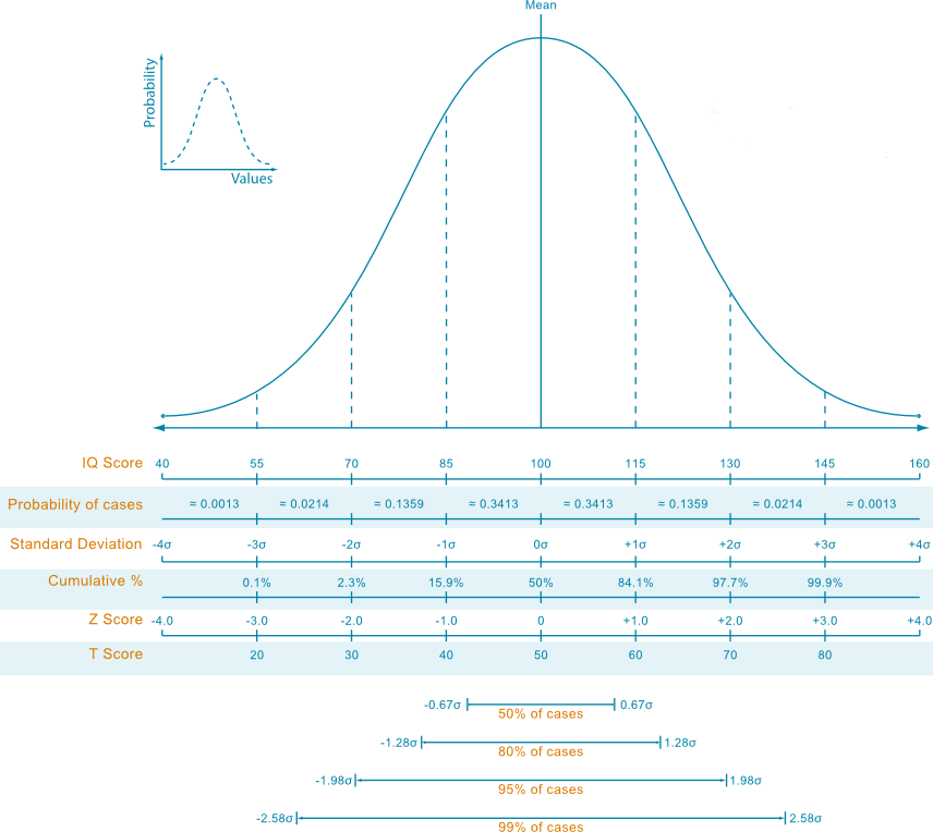
We notice that the median of our player’s population scores a TQ equal to 100.
(median_value <- median(slam_winners$WINS))
[1] 2
(deviation_median <- (log(median_value) - mean_norm)/sd_norm)
[1] -0.01444343
round(100 + 15*deviation_median)
[1] 100
We now compute the Tennis Quotients (TQ) for leading champions.
(Federer_TQ <- round(100 + 15*deviation_19))
[1] 142
(Nadal_TQ <- round(100 + 15*deviation_16))
[1] 138
(Sampras_TQ <- round(100 + 15*deviation_14))
[1] 136
And what about for example 7 times Grand Slam tournament winner?
(deviation_7 <- (log(7) - mean_norm)/sd_norm)
[1] 1.53931
TQ_7wins <- round(100 + 15*deviation_7)
[1] 123
Let us then compute the Tennis Quotients (TQ) for all our tennis Grand Slam tournaments winners.
tq_compute <- function(x) {
  deviation_x <- (log(x) - mean_norm)/sd_norm
  round(100 + 15*deviation_x)
}
slam_winners = slam_winners %>% mutate(TQ = tq_compute(WINS))
kable(slam_winners)
| RANK|PLAYER                      | WINS| LAST_WIN_YEAR|  TQ|
|----:|:---------------------------|----:|-------------:|---:|
|    1|Roger Federer               |   19|          2017| 142|
|    2|Rafael Nadal                |   16|          2017| 138|
|    3|Pete Sampras                |   14|          2002| 136|
|    4|Novak Djokovic              |   12|          2016| 133|
....
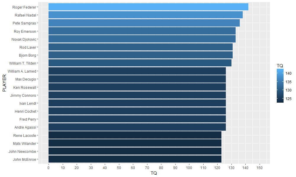
We then visualize the top twenty Grand Slam tournaments champions.
ggplot(data=slam_winners[1:20,], aes(x=reorder(PLAYER, TQ), y=TQ, fill = TQ)) +
  geom_bar(stat ="identity") + coord_flip() +
  scale_y_continuous(breaks = seq(0,150,10), limits = c(0,150)) +
  xlab("PLAYER")
Gives this plot.
Conclusions
The answers to our initial questions:
– The log-normal distribution
– Based upon the fitted distribution and taking advantage ofplnorm()orpnorm()stats package functions, probabilities have been computed
– A linear increase is a very good fit for that, resulting in significative regression coefficients and high R-squared values
– Yes, we defined the Tennis Quotient similarly to the Intellectual Quotient and show the resulting leaderboard. Federer is confirmed “genius” in that respect, however, a few other very talented players are not that far from him.
If you have any questions, please feel free to comment below.
References
- [1] tennis-grand-slam-winners_end2017