In Randomized Controlled Trials (RCTs), a “Pre” measurement is often taken at baseline (before randomization), and treatment effects are measured at one or more time point(s) after randomization (“Post” measurements). There are many ways to take the baseline measurement into account when comparing 2 groups in a classic pre-post design with one post measurement. Here, I will discuss the constrained longitudinal data analysis (cLDA).
In this post several strategies were discussed, including:
- The delta approach: a comparison of the “delta's” (post measurement minus baseline measurement) using a independent samples t-test.
- The ANCOVA: A regression model with the pre measurement and group as predictors, and the post measurement as outcome variabele.
In this tutorial, we will apply the constrained longitudinal data analysis (cLDA) model in R.
LDA (as defined in Liu, 2009) is a mixed model approach where both baseline measurements and post measurements are modeled as dependent variables. The model includes at least Group, Time and their interaction Group:Time as predictors. We're specifically interested in the interaction term, telling us whether the changes in mean response over time differ accross groups.
In cLDA, the group means are assumed to be equal at baseline (hence the “constrained” in cLDA), which is a reasonable assumption in a randomized trial. As described below, this strategy is an important exception of the rule that an interaction should not be included in a model without its main effects.
In Liu, 2009 several advantages of this method are listed:
- In contrast to the ANCOVA and delta approach, all subjects with at least one measurement (baseline or post-randomization) are included in the analysis.
- The models can easily be extended to 3 or more repeated measures.
- It is possible to model the correlation between baseline and post measures differently for different treatment groups.
I'll share with you how to perform this analysis in R. At the end of the post you'll find a short section about non-randomized experiments/studies.
Simulating the data
Data were created using the simstudy package. Each subject has equal chance to be assigned to either the Control group or the Experimental group. Both Pre and Post measurements are normally distributed. The assignment has no influence on the pre measurement. The post measurement depends on Group (Exp or Con) and on the baseline measurement (Pre).
library(simstudy)
tdef <- defData(varname = "Group", dist = "binary",
                formula = 0.5,  id = "Id")
tdef <- defData(tdef, varname = "Pre", dist = "normal",
                formula = 7, variance = 10)
tdef <- defData(tdef, varname = "Post", dist = "normal",
                formula = "Pre + 0.1 + 1.05* Group", variance =3 )
set.seed(123)
dtTrial <- genData(150, tdef)
dtTrial$Group <- factor(dtTrial$Group, levels=c(1,0),
labels=c("Exp", "Con"))
library(knitr)
kable(head(dtTrial))
| Id | Group | Pre | Post |
|---|---|---|---|
| 1 | Con | 10.243141 | 10.446631 |
| 2 | Exp | 6.099469 | 6.029072 |
| 3 | Con | 3.139752 | 1.997493 |
| 4 | Exp | 7.573332 | 10.255592 |
| 5 | Exp | 6.560787 | 5.951729 |
| 6 | Con | 7.018228 | 10.504896 |
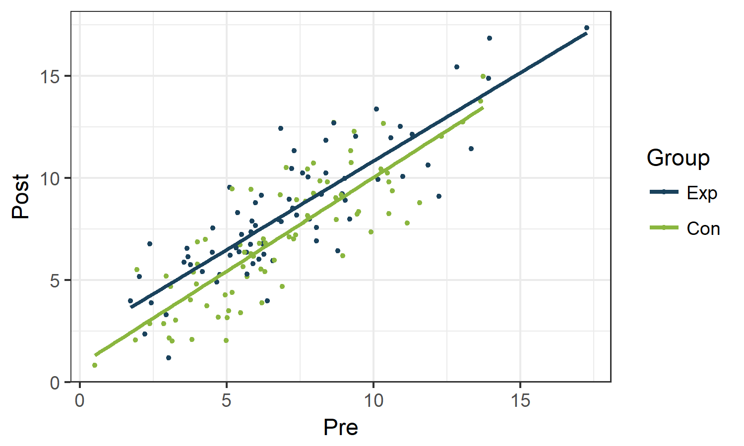
A dot plot of Post versus Pre visualizes the correlation between both time points:
library(ggplot2)
fav.col=c("#1A425C", "#8AB63F")
ggplot(dtTrial, aes (x=Pre,y=Post, col=Group)) +
        geom_point() + geom_smooth(method="lm", se=FALSE) +
        scale_color_manual(values=fav.col) + theme_bw()
Gives this plot:
From wide to long format
When applying mixed models, the baseline measurement is seen as part of the outcome vector. All measurements (pre and post) should appear in one column (the variable Outcome ). Tidyverse's gather() function is one of the many ways to do the job. In this example the columns Pre and Post are “gathered” in a column called Outcome (=value). The new variable called Time (=key) will show us whether it concerns a pre or post measurement.
library (tidyverse)
dtTrial_long <- gather(data=dtTrial, key=Time, value=Outcome,
        Pre:Post, factor_key=TRUE)
kable(head(arrange(dtTrial_long, Id), 10))
| Id | Group | Time | Outcome |
|---|---|---|---|
| 1 | Con | Pre | 10.243141 |
| 1 | Con | Post | 10.446631 |
| 2 | Exp | Pre | 6.099469 |
| 2 | Exp | Post | 6.029072 |
| 3 | Con | Pre | 3.139752 |
| 3 | Con | Post | 1.997493 |
| 4 | Exp | Pre | 7.573332 |
| 4 | Exp | Post | 10.255592 |
| 5 | Exp | Pre | 6.560787 |
| 5 | Exp | Post | 5.951729 |
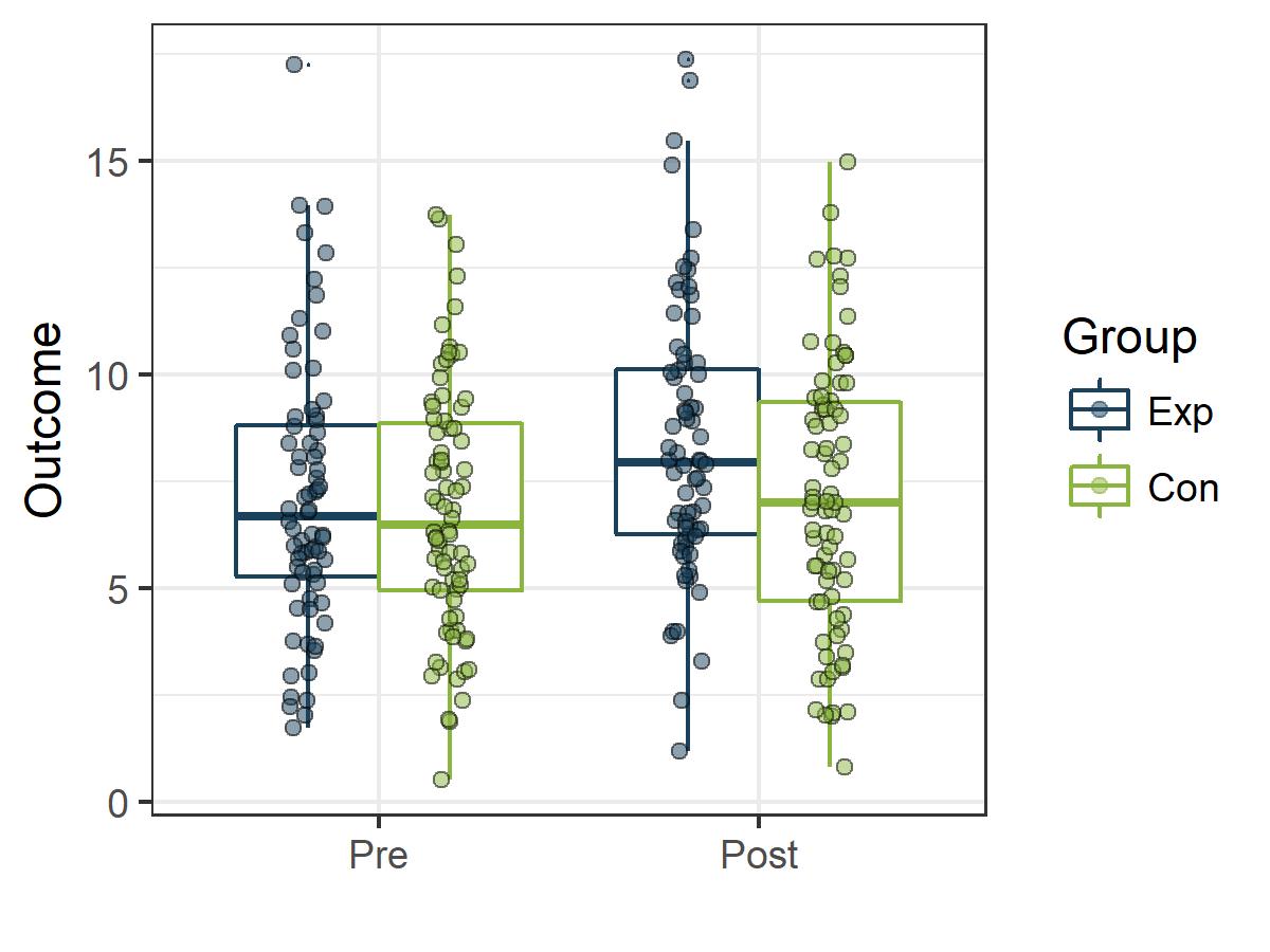
Once the data are structured in a “long” format the creation of a boxplot to visualize the data is simple:
library(ggplot2)
boxp <- ggplot (dtTrial_long , aes(x=Time,y=Outcome, col=Group))+
        geom_boxplot(outlier.size = 0 ) +
        geom_point(aes(fill=Group, col=NULL),shape=21, alpha=0.5, size=2,
        position = position_jitterdodge(jitter.width = 0.2)) +
        scale_fill_manual(values=fav.col) +
        scale_color_manual(values=fav.col) +
        theme_bw() + xlab("")

boxp
Gives this plot:
Applying constrained longitudinal data analysis (cLDA)
The gls() function of the nlme package can be used to apply LDA modelling.
Fixed part
The terms of the most basic cLDA model are Time and Time * Group . By omitting Group , there is no term allowing for a difference in means at baseline between the groups. Consequently, the baseline means are assumed to be equal.
However, a general rule in regression modelling is that when adding an interaction to the model, the lower ranked effects should also be included in the model. For this reason, R will automatically include Time and Group as main effects in the model when including the interaction term Time*Group.
To avoid to have Group as the main effect in our model, we will create an alternative model matrix: Xalt.
X <- model.matrix(~ Time * Group, data = dtTrial_long)
colnames(X)
[1] "(Intercept)"       "TimePost"          "GroupCon"
[4] "TimePost:GroupCon"
Xalt <- X[, c("TimePost", "TimePost:GroupCon")]
colnames(Xalt)
[1] "TimePost"          "TimePost:GroupCon"
Random part
The standard deviations and correlations that should be estimated are defined by the constant variance function varIdent(). By setting weights = varIdent(form = ~ 1 | Time) a separate standard deviation will be estimated for each time point and a seperate correlation will be estimated for each pair of time points (= unstructured variance covariance matrix). Applied to our example, we expect an estimated standard deviation for Time=Pre, an estimated standard deviation for Time=Post and one estimated correlation between the pre- and post measurements of the same subject.
Remark: By setting weights = varIdent(form = ~ 1 | Time:Group), a separate variance is estimated for each combination of Group and Time (Pre-Exp Post-Exp Pre-Con Post-Con ).
The argument correlation=corSymm (form = ~ 1 | Id) defines the subject levels. The correlation structure is assumed to apply only to observations within the same subject (in our example: Id); observations from different subjects (a different value for Id) are assumed to be uncorrelated.
library(nlme)

clda_gls <- gls(Outcome ~ Xalt,
weights = varIdent(form = ~ 1 | Time),
correlation=corSymm (form = ~ 1 | Id),
data = dtTrial_long)
summary(clda_gls)
Generalized least squares fit by REML
  Model: Outcome ~ Xalt
  Data: dtTrial_long
       AIC     BIC    logLik
  1358.307 1380.47 -673.1537

Correlation Structure: General
 Formula: ~1 | Id
 Parameter estimate(s):
 Correlation:
  1
2 0.842
Variance function:
 Structure: Different standard deviations per stratum
 Formula: ~1 | Time
 Parameter estimates:
     Pre     Post
1.000000 1.059605

Coefficients:
                          Value Std.Error   t-value p-value
(Intercept)            6.978858 0.2461488 28.352190   0e+00
XaltTimePost           1.240246 0.2047301  6.057956   0e+00
XaltTimePost:GroupCon -0.958945 0.2815211 -3.406297   7e-04

 Correlation:
                      (Intr) XltTmP
XaltTimePost          -0.129
XaltTimePost:GroupCon  0.000 -0.715

Standardized residuals:
        Min          Q1         Med          Q3         Max
-2.20538393 -0.65214666 -0.09411877  0.63654736  3.40671592

Residual standard error: 3.014695
Degrees of freedom: 300 total; 297 residual
The p-value for the interaction effect (the effect of interest here) is 0.0007: the change in mean over time differs significantly between groups. The estimated difference in change is -0.95 (SE: 0.28) (Con increases 0.95 less then Exp).
The estimated correlation between Pre and Post is 0.842. The estimated standard deviation for the Pre measurement is 3.01 and the estimated standard devaition for the Post measurement is 1.059 * 3.01.
We can obtain predicted means using the gls() function. As expected, the predicted value is the same for both groups at baseline ( Time == Pre).
predictions<- cbind( dtTrial_long,clda_gls$fitted)
| Id | Group | Time | Outcome | clda_gls$fitted |
|---|---|---|---|---|
| 1 | Con | Pre | 10.243141 | 6.978858 |
| 1 | Con | Post | 10.446631 | 7.260160 |
| 2 | Exp | Pre | 6.099469 | 6.978858 |
| 2 | Exp | Post | 6.029072 | 8.219104 |
Preferably we also report the confidence intervals. That's where the Gls() function of the rms package comes in. It uses exactly the same arguments as the gls() function, leading to exactly the same predictions. But the Gls() function allows us to create confidence intervals.
library(rms)
clda_Gls <- Gls(Outcome ~ Xalt,
        weights = varIdent(form = ~ 1 | Time),
        correlation=corSymm (form = ~ 1 | Id),
        data = dtTrial_long)

predictions <- cbind(dtTrial_long,
predict (clda_Gls, dtTrial_long, conf.int=0.95))
Now we do obtain 95% confidence intervals:
| Id | Group | Time | Outcome | linear.predictors | lower | upper |
|---|---|---|---|---|---|---|
| 1 | Con | Pre | 10.243141 | 6.978858 | 6.496415 | 7.461301 |
| 1 | Con | Post | 10.446631 | 7.260160 | 6.684425 | 7.835894 |
| 2 | Exp | Pre | 6.099469 | 6.978858 | 6.496415 | 7.461301 |
| 2 | Exp | Post | 6.029072 | 8.219104 | 7.632889 | 8.805319 |
Plotting the confidence intervals
First attempt at the visualization of the estimated means and their 95% confidence intervals:
pd <- position_dodge(.1)
limits <- aes(ymax = upper , ymin=lower, shape=Group)

pCI1 <- ggplot(predictions, aes( y=linear.predictors, x=Time)) +
        geom_errorbar(limits, width= 0.1 , position=pd) +
        geom_line(aes(group=Group, y=linear.predictors), position=pd) +
        geom_point(position=pd, aes( fill=Group), shape=21, size=4) +
        scale_fill_manual(values=c( "black", "white")) +
        theme_bw() +
        theme(panel.grid.major = element_blank(), legend.title=element_blank(),
        text=element_text(size=14), legend.position="bottom") +
        xlab("") +
        ylab("Estimated mean with corresponding 95% CI")
pCI1
Gives this plot:
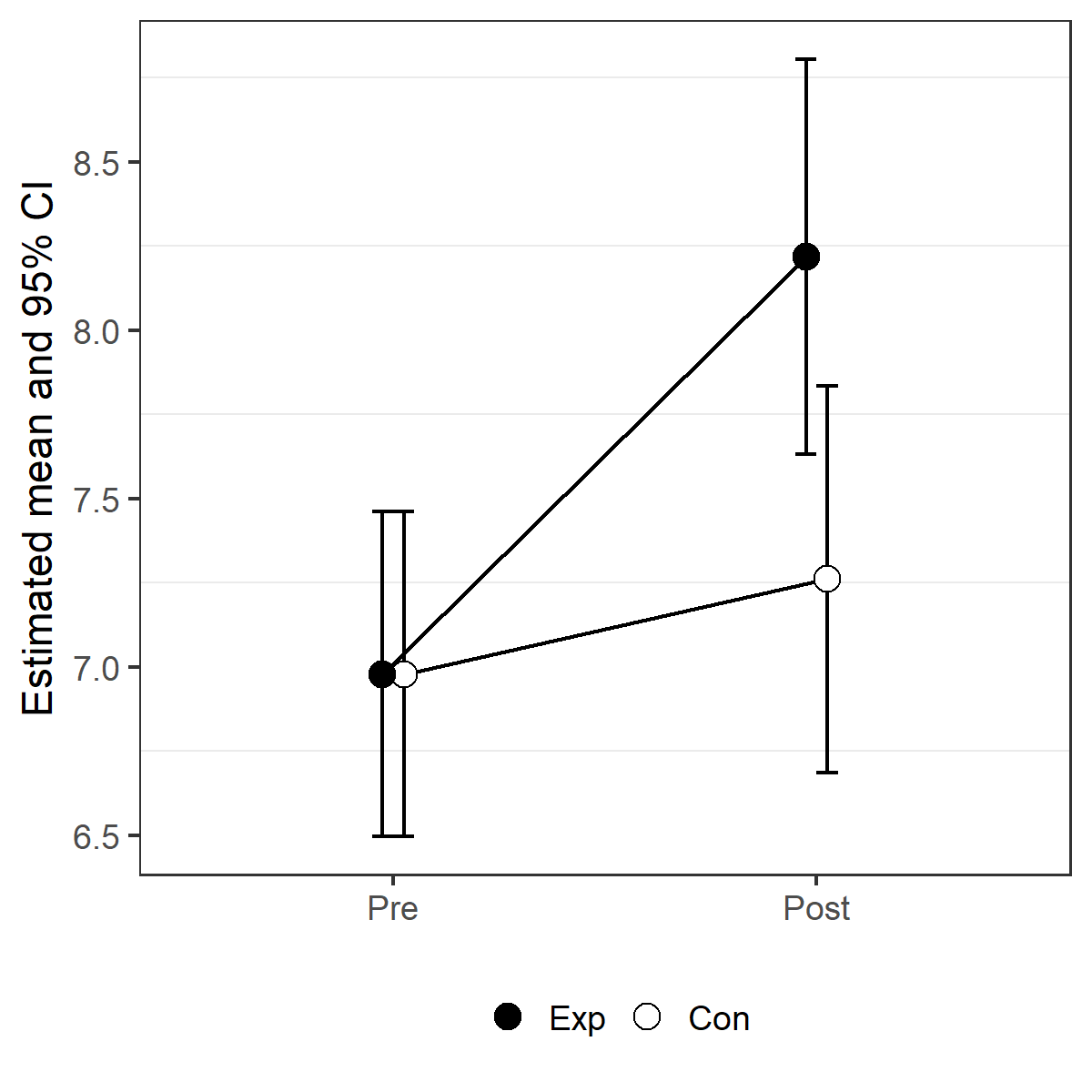
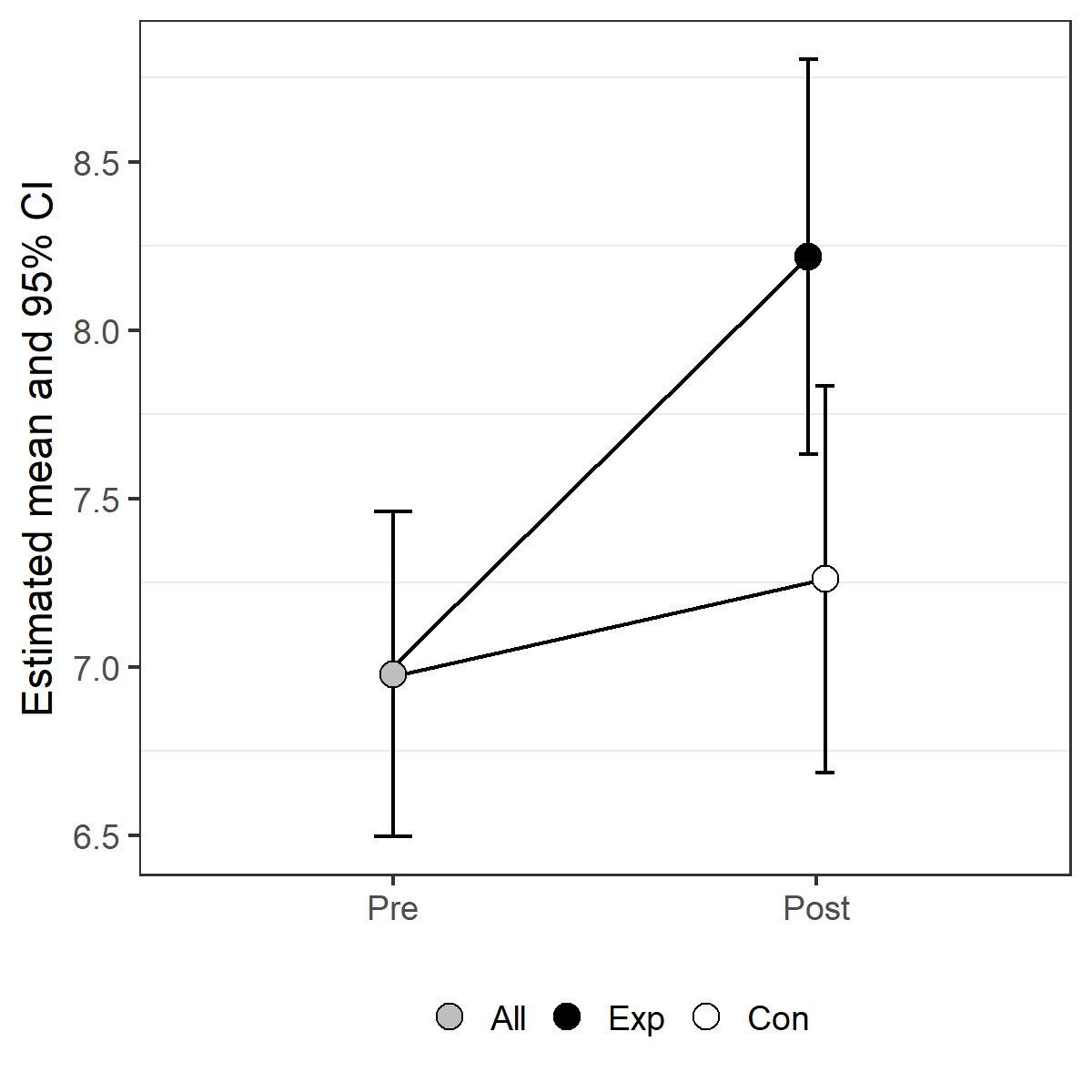
To my opinion, this plot can be misleading. One estimated mean is presented by 2 different dots. I prefer to create the factor Group2 and remake the plot.
predictions$Group2<- factor(predictions$Group,
        levels= c("All", "Exp", "Con"))
predictions$Group2 [predictions$Time=="Pre"] <- "All"

pd <- position_dodge(.08)
limits <- aes(ymax = upper , ymin=lower, shape=Group2)

pCI <- ggplot(predictions, aes( y=linear.predictors, x=Time)) +
        geom_errorbar(limits, width=0.09,position=pd) +
        geom_line(aes(group=Group, y=linear.predictors), position=pd)+
        geom_point(position=pd, aes( fill=Group2), shape=21, size=4) +
        scale_fill_manual(values=c("grey", "black", "white")) +
        theme_bw() +
        theme(panel.grid.major = element_blank(), legend.title=element_blank(),
        text=element_text(size=14), legend.position="bottom") +
        xlab ("") +
        ylab("Estimated mean with corresponding 95% CI")
pCI
Gives this plot:
In the case of non-randomized experiments
In the case of non-randomized experiments or studies an equal mean at baseline cannot be assumed. Consequently, applying constrained LDA is not appropriate. It is, however, possible to perform an LDA (without the constraint). By including Group in the model (next to Time and the interaction term Group:Time ), the baseline means are allowed to differ between groups.
There's no need to create the alternative model matrix Xalt in that situation. (Xalt can thus be replaced by Group:Time )
The remaining arguments (random part of the model) doesn't differ from the model we presented for cLDA.
References
References LDA and cLDA:
- Fitzmaurice, Garrett M., et al. Applied Longitudinal Analysis. John Wiley & Sons, 2004.
- Liu GF, Lu K, Mogg R, et al. Should baseline be a covariate or dependent variable in analyses of change from baseline in clinical trials? Stat Med 2009; 28: 2509-2530.
Reference Gls() function of the rms package:
- Pinheiro J, Bates D (2000): Mixed effects models in S and S-Plus. New York: Springer-Verlag.
Great approach! However, is it possible to use anova on the model to get 1 p-value for the interaction (in case you have multiple test phases and hence multiple interaction terms in the summary table)? Doing it this way you get one p-value for Xalt, and I haven’t figured out a way to get the regular anova table. Many thanks!
Great article, thank you! DO you know if it’s possible to use the lme4 package for cLDA modelling ? It’s my usual choice for (generalized) mixed models, but it seems that the framework is not as flexible as the nlme package in terms of specifying the structure of the variance-covariance matrix.
Could this approach be implemented when there is an additional fixed effect for clustering (e.g., a variable for classroom)?