Table 1 and the Characteristics of Study Population

In research, and especially in medical research, we describe the characteristics of our study population through Table 1. Table 1 reports the mean for continuous variables and the proportion for categorical variables. For example, we say that the mean systolic blood pressure in our study population is 145 mmHg, or that 30% of participants are smokers. It is called Table 1 because it is usually the first table in the manuscript.

Creating Table 1 can be very time-consuming. Imagine that we have 10 variables (e.g. age, gender, etc.) for 3 groups, and for each variable we compute the mean (standard deviation) or the number of participants (proportion); in the end, we would have to fill in 60 numbers in the table. Moreover, we usually export the table from R to Microsoft Word, and we are prone to making mistakes when copy/pasting. Therefore, I searched for a simple and comprehensive way to make Table 1 with R, and found two very interesting packages: “tableone” and “ReporteRs”. The tableone package, created by Kazuki Yoshida and Justin Bohn, is used to create Table 1 in R. The ReporteRs package, created by David Gohel, is what I use in this post to export the table from R to Microsoft Word.

Create Table 1

I simulated a dataset by using the functions rnorm() and sample(). You can download this simulated dataset to your desktop to replicate this post. To learn how to load your dataset into R, read this post.

dt <- read.csv(file.choose(), header=TRUE, sep=",")
head(dt) 
  Age Gender Cholesterol SystolicBP  BMI Smoking Education
1 67.9 Female       236.4      129.8 26.4     Yes      High
2 54.8 Female       256.3      133.4 28.4      No    Medium
3 68.4   Male       198.7      158.5 24.1     Yes      High
4 67.9   Male       205.0      136.0 19.9      No       Low
5 60.9   Male       207.7      145.4 26.7      No    Medium
6 44.9 Female       222.5      130.6 30.6      No       Low

Now I will use the tableone package to create Table 1. First I load the package and create the list of variables that I want to include in Table 1. Then I define which of them are categorical variables.

#Load package
library(tableone)

#Create a variable list which we want in Table 1
listVars <- c("Age", "Gender", "Cholesterol", "SystolicBP", "BMI", "Smoking", 
"Education")

#Define categorical variables
catVars <- c("Gender","Smoking","Education")

My first interest is to make Table 1 for the total population.

#Total Population
table1 <- CreateTableOne(vars = listVars, data = dt, factorVars = catVars)
table1
                         Overall       
  n                          250        
  Age (mean (sd))          57.50 (7.85) 
  Gender = Male (%)          107 (42.8) 
  Cholesterol (mean (sd)) 224.12 (24.90)
  SystolicBP (mean (sd))  145.51 (10.08)
  BMI (mean (sd))          26.79 (4.37) 
  Smoking = Yes (%)           72 (28.8) 
  Education (%)                         
     High                    108 (43.2) 
     Low                      71 (28.4) 
     Medium                   71 (28.4)

Often, however, I am interested in creating Table 1 separately for men and women, so I can compare their means and proportions. To do this, I run the code below, which stratifies the table by gender and adds a p-value for the comparison between groups.

# Removing Gender from list of variables 
listVars <- c("Age", "Cholesterol", "SystolicBP", "BMI", "Smoking", "Education")
table1 <- CreateTableOne(listVars, dt, catVars, strata = c("Gender"))
table1
                         Stratified by Gender
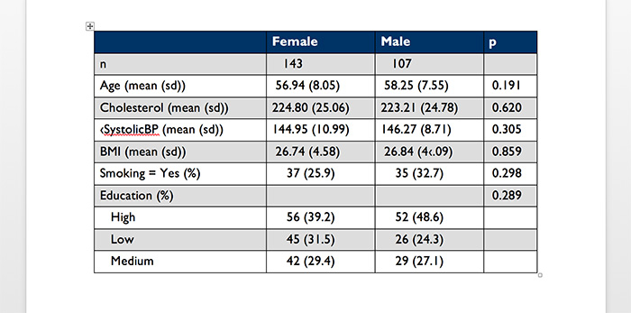
                          Female         Male           p      test
  n                          143            107                    
  Age (mean (sd))          56.94 (8.05)   58.25 (7.55)   0.191     
  Cholesterol (mean (sd)) 224.80 (25.06) 223.21 (24.78)  0.620     
  SystolicBP (mean (sd))  144.95 (10.99) 146.27 (8.71)   0.305     
  BMI (mean (sd))          26.74 (4.58)   26.84 (4.09)   0.859     
  Smoking = Yes (%)           37 (25.9)      35 (32.7)   0.298     
  Education (%)                                          0.289     
     High                     56 (39.2)      52 (48.6)             
     Low                      45 (31.5)      26 (24.3)             
     Medium                   42 (29.4)      29 (27.1) 

You can do a lot more with the tableone package. For example, you can compute the median and interquartile range for non-normally distributed variables, and run different tests to compare the groups.

Export Table 1 from R to Microsoft Word

Now that Table 1 is ready, I want to transfer it to a Microsoft Word document. For this purpose I use the function FlexTable() from the ReporteRs package. I found a very good script on StackOverflow to achieve this task, and I am sharing the code below (credits to the author on StackOverflow).

table1 <- print(table1)

# Load the packages
library(ReporteRs)
library(magrittr)

# The script
docx( ) %>% 
     addFlexTable(table1 %>%
     FlexTable(header.cell.props = cellProperties( background.color = "#003366"),
               header.text.props = textBold( color = "white" ),
               add.rownames = TRUE ) %>%
               setZebraStyle( odd = "#DDDDDD", even = "#FFFFFF" ) ) %>%
     writeDoc(file = "table1.docx")

This creates a file named table1.docx in your working directory. Finally, you will have Table 1 ready for submission.
Here is a screenshot of my Table 1:

If you have any comments or feedback, feel free to post a comment below.