In time series analysis, structural changes represent shocks impacting the evolution with time of the data generating process. That is relevant because one of the key assumptions of the Box-Jenkins methodology is that the structure of the data generating process does not change over time. How can structural changes be identified ? The strucchange package can help in that and the present tutorial shows how.
R Packages
suppressPackageStartupMessages(library(strucchange))
suppressPackageStartupMessages(library(fUnitRoots))
suppressPackageStartupMessages(library(astsa))
Basic Data Exploration
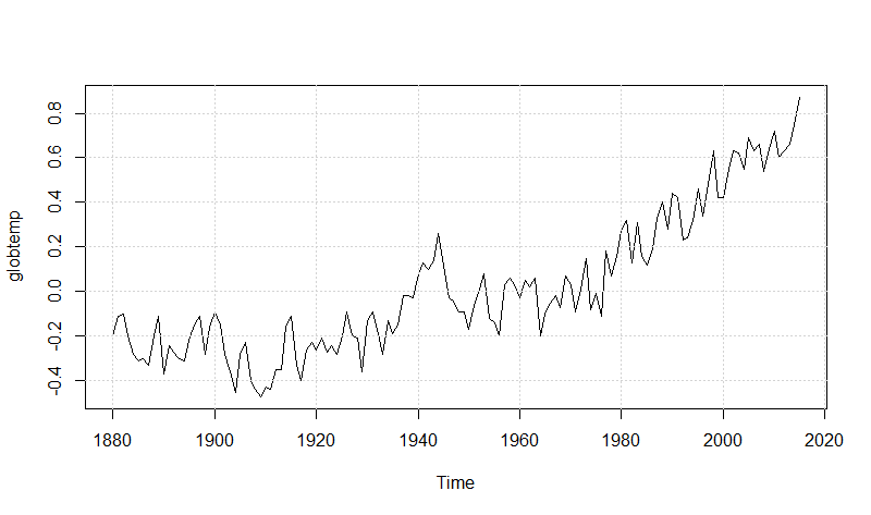
We are going to do a basic exploration of the globtemp time series as available within the astsa package. The globtemp dataset reports the deviation (in degrees centigrade) from [1951-1980] global mean land-ocean temperature. Let us have a look at it.
data("globtemp")
globtemp
Time Series:
Start = 1880
End = 2015
Frequency = 1
  [1] -0.20 -0.11 -0.10 -0.20 -0.28 -0.31 -0.30 -0.33 -0.20 -0.11 -0.37 -0.24 -0.27
 [ t14] -0.30 -0.31 -0.22 -0.15 -0.11 -0.28 -0.16 -0.09 -0.15 -0.28 -0.36 -0.45 -0.28
 [27] -0.23 -0.40 -0.44 -0.47 -0.43 -0.44 -0.35 -0.35 -0.16 -0.11 -0.33 -0.40 -0.26
 [40] -0.23 -0.26 -0.21 -0.27 -0.24 -0.28 -0.20 -0.09 -0.20 -0.21 -0.36 -0.13 -0.09
 [53] -0.17 -0.28 -0.13 -0.19 -0.15 -0.02 -0.02 -0.03  0.08  0.13  0.10  0.14  0.26
 [66]  0.12 -0.03 -0.04 -0.09 -0.09 -0.17 -0.06  0.01  0.08 -0.12 -0.14 -0.20  0.03
 [79]  0.06  0.03 -0.03  0.05  0.02  0.06 -0.20 -0.10 -0.05 -0.02 -0.07  0.07  0.03
 [92] -0.09  0.01  0.15 -0.08 -0.01 -0.11  0.18  0.07  0.16  0.27  0.32  0.13  0.31
[105]  0.16  0.12  0.19  0.33  0.40  0.28  0.44  0.42  0.23  0.24  0.32  0.46  0.34
[118]  0.48  0.63  0.42  0.42  0.55  0.63  0.62  0.55  0.69  0.63  0.66  0.54  0.64
[131]  0.72  0.60  0.63  0.66  0.75  0.87
summary(globtemp)
    Min.  1st Qu.   Median     Mean  3rd Qu.     Max.
-0.47000 -0.21000 -0.07500  0.01838  0.18250  0.87000
plot(globtemp)
grid()
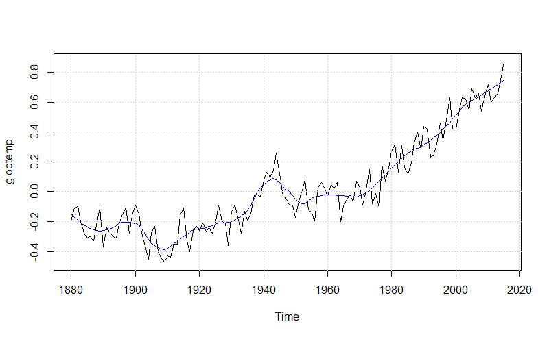
We can see a remarkable increase of the temperature deviations in the last decades. The globtemp time series appears to be non stationary due basically to the last decades upward trend. A plot of globtemp against its smoothed fit may help in understand better.
tt <- 1:length(globtemp)
fit <- ts(loess(globtemp ~ tt, span = 0.2)$fitted, start = 1880, frequency = 1)
plot(globtemp, type='l')
lines(fit, col = 4)
grid()
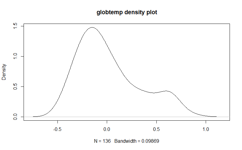
The globtemp density plot is herein shown.
plot(density(globtemp), main = "globtemp density plot")
We are going to run the Augmented Dickey-Fuller test with type = “ct” having the following models, null-hypothesis and test statistics.
$$
\begin{equation}
\begin{cases}
\ Model:\ \Delta y_{t}\ =\ a_{0}+ \gamma y_{t-1} + a_{2}t\ + \epsilon_{t} \\
\\
H_{0}: \gamma = 0\ \ \ \ \ test\ statistics: \tau_{3} \\
\\
H_{0}: \gamma = a_{2} = 0\ \ \ \ \ test\ statistics: \phi_{3} \\
\\
H_{0}: \ a_{0} = \gamma = a_{2} = 0\ \ \ \ \ test\ statistics: \phi_{2} \\
\end{cases}
\end{equation}
$$
See ref. [3] for details about the Dickey-Fuller test and its report as output by the urdfTest() function within the fUnitRoots package.
urdftest_lag = floor(12*(length(globtemp)/100)^0.25) # long
urdfTest(globtemp, lags = urdftest_lag, type = c("ct"), doplot = FALSE)
Title:
 Augmented Dickey-Fuller Unit Root Test

Test Results:

  Test regression trend

  Call:
  lm(formula = z.diff ~ z.lag.1 + 1 + tt + z.diff.lag)

  Residuals:
        Min        1Q    Median        3Q       Max
  -0.233454 -0.061206  0.000907  0.067984  0.196946

  Coefficients:
                Estimate Std. Error t value Pr(>|t|)
  (Intercept)  -0.066984   0.049114  -1.364  0.17546
  z.lag.1      -0.104138   0.086354  -1.206  0.23048
  tt            0.001213   0.000651   1.863  0.06517 .
  z.diff.lag1  -0.273952   0.119332  -2.296  0.02362 *
  z.diff.lag2  -0.324109   0.120821  -2.683  0.00845 **
  z.diff.lag3  -0.263840   0.122262  -2.158  0.03314 *
  z.diff.lag4  -0.029046   0.123184  -0.236  0.81404
  z.diff.lag5  -0.164546   0.124910  -1.317  0.19052
  z.diff.lag6  -0.121042   0.124239  -0.974  0.33210
  z.diff.lag7  -0.063802   0.122548  -0.521  0.60369
  z.diff.lag8   0.043304   0.119004   0.364  0.71665
  z.diff.lag9  -0.088910   0.116985  -0.760  0.44891
  z.diff.lag10  0.071604   0.111461   0.642  0.52197
  z.diff.lag11 -0.049646   0.102584  -0.484  0.62940
  z.diff.lag12 -0.037257   0.095916  -0.388  0.69846
  ---
  Signif. codes:  0 ‘***’ 0.001 ‘**’ 0.01 ‘*’ 0.05 ‘.’ 0.1 ‘ ’ 1

  Residual standard error: 0.09935 on 108 degrees of freedom
  Multiple R-squared:  0.2657,	Adjusted R-squared:  0.1705
  F-statistic: 2.791 on 14 and 108 DF,  p-value: 0.001403


  Value of test-statistic is: -1.2059 2.8535 2.3462

  Critical values for test statistics:
        1pct  5pct 10pct
  tau3 -3.99 -3.43 -3.13
  phi2  6.22  4.75  4.07
  phi3  8.43  6.49  5.47
By comparing the test statistics with the critical values at 5% significance level we cannot reject any of the null hypothesis. As a consequence, the unit root hypothesis cannot be rejected. Since in case of structural breaks, the Dickey Fuller test is biased toward the non rejection of the null hypothesis (ref. [3]), we run the KPSS test having the trend stationarity hypothesis as null (i.e. deterministic trend with stationary residuals).
urkpssTest(globtemp, type = c("tau"), lags = c("long"),  doplot = FALSE)
Title:
 KPSS Unit Root Test

Test Results:

  Test is of type: tau with 12 lags.

  Value of test-statistic is: 0.2114

  Critical value for a significance level of:
                  10pct  5pct 2.5pct  1pct
  critical values 0.119 0.146  0.176 0.216
We reject the trend stationarity hypothesis based on the resulting test statistics compared with their significance levels.
Structural Changes Detection
Bai and Perron established a general methodology for estimating breakpoints and their associated confidence intervals in OLS regression employing dynamic programming. In that way, it is possible to find m breakpoints that minimize the residual sum of square (RSS) associated to a model with m+1 segments given some minimal segment size of h·n observations. The h bandwidth parameter is chosen by the user typically equal to 0.1 or 0.15. Since the number of breakpoints m is not known in advance, it is necessary to compute the optimal breakpoints for m = 0, 1, … breaks and choose the model that minimizes some information criterion such as BIC (ref. [1]). That model selection strategy is available within breakpoints() function of the strucchange R package (ref. [2]).
Structural Changes Analysis
In the following, we determine the globtemp time series structural changes dates, if any. Such analysis is named as “dating structural changes (breaks)”. Specifically, we are looking for:
* level structural changes
* trend structural changes
* polinomial fit structural changes
* auto-regressive model structural changes
Level Structural Changes
Level structural changes can be determined with the help of the following formula:
globtemp ~ 1
We remark that any structural change analysis should be run against regressors which are significative in terms of time series fit. At that purpose we run:
summary(lm(globtemp ~ 1))
Call:
lm(formula = globtemp ~ 1)

Residuals:
     Min       1Q   Median       3Q      Max
-0.48838 -0.22838 -0.09338  0.16412  0.85162

Coefficients:
            Estimate Std. Error t value Pr(>|t|)
(Intercept)  0.01838    0.02721   0.676      0.5

Residual standard error: 0.3173 on 135 degrees of freedom
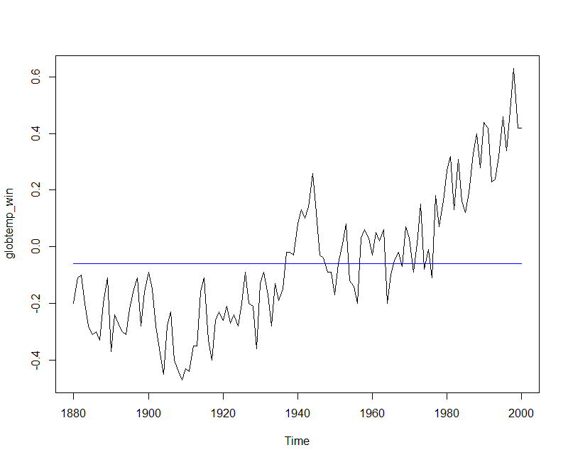
The intercept coefficient is not significative, likely due to the upward trend observable in the last decades. We then shorten our time series and run again the same regression.
globtemp_win <- window(globtemp, end = 2000)
lev_fit <- lm(globtemp_win ~ 1)
summary(lev_fit)
Call:
lm(formula = globtemp_win ~ 1)

Residuals:
     Min       1Q   Median       3Q      Max
-0.41017 -0.17017 -0.04017  0.13983  0.68983

Coefficients:
            Estimate Std. Error t value Pr(>|t|)
(Intercept) -0.05983    0.02161  -2.769  0.00652 **
---
Signif. codes:  0 ‘***’ 0.001 ‘**’ 0.01 ‘*’ 0.05 ‘.’ 0.1 ‘ ’ 1

Residual standard error: 0.2377 on 120 degrees of freedom
The intercept coefficient is now reported as significant. Let us plot the time series against the fit.
plot(globtemp_win)
lines(ts(fitted(lev_fit), start = 1880, frequency = 1), col = 4)
We go on with the search for structural changes.
globtemp_brk <- breakpoints(globtemp_win ~ 1, h = 0.1)
summary(globtemp_brk)
	 Optimal (m+1)-segment partition:

Call:
breakpoints.formula(formula = globtemp_win ~ 1, h = 0.1)

Breakpoints at observation number:

m = 1                        97
m = 2               57       100
m = 3               57       97  109
m = 4      22 34    57       100
m = 5      22 34    57       97  109
m = 6      22 34    57 69    97  109
m = 7      22 34    57 69 81 97  109
m = 8      22 34 46 58 70 85 97  109
m = 9   12 24 36 48 60 72 84 97  109

Corresponding to breakdates:

m = 1                                      1976
m = 2                       1936           1979
m = 3                       1936           1976 1988
m = 4        1901 1913      1936           1979
m = 5        1901 1913      1936           1976 1988
m = 6        1901 1913      1936 1948      1976 1988
m = 7        1901 1913      1936 1948 1960 1976 1988
m = 8        1901 1913 1925 1937 1949 1964 1976 1988
m = 9   1891 1903 1915 1927 1939 1951 1963 1976 1988

Fit:

m   0         1         2         3         4         5         6         7         8         9
RSS    6.7814    2.7965    1.3933    1.2582    1.1600    1.0249    0.9663    0.9606    0.9760    1.1440
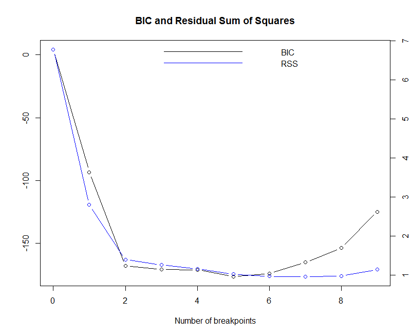
BIC    4.3002  -93.2918 -168.0043 -170.7502 -170.9914 -176.3777 -173.9182 -165.0385 -153.5225 -124.7135
Above the results of finding m = 1..9 breakpoints with associated dates and {RSS, BIC} metrics. The minimum value of BIC is reached for m = 5. We plot the breakpoint() function output to gather a visual understanding of.
plot(globtemp_brk)
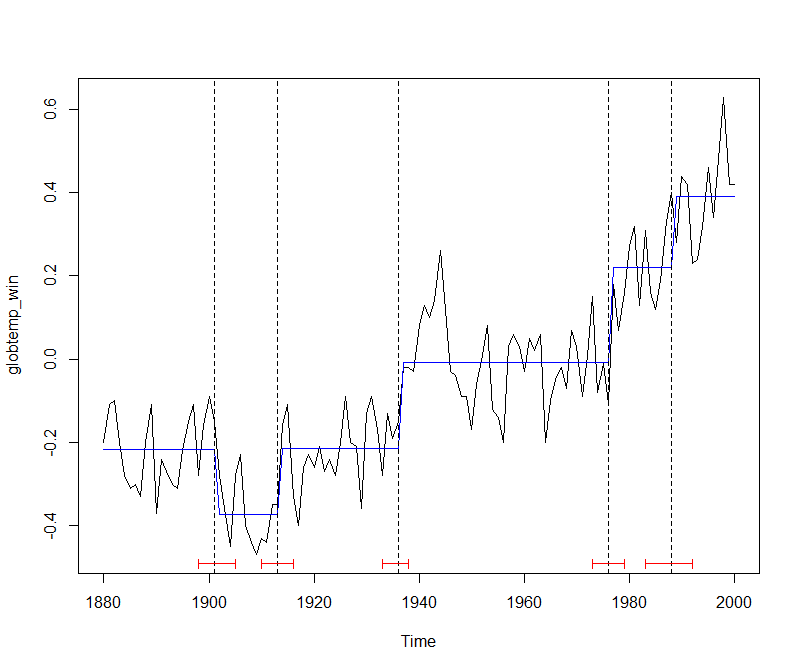
The plot of the observed and fitted time series, along with confidence intervals for the breakpoints, is given by:
plot(globtemp_win)
lines(fitted(globtemp_brk, breaks = 5), col = 4)
lines(confint(globtemp_brk, breaks = 5))
The break dates are:
breakdates(globtemp_brk, breaks = 5)
[1] 1901 1913 1936 1976 1988
Level breaks coefficients:
coef(globtemp_brk, breaks = 5)
            (Intercept)
1880 - 1901  -0.2177273
1902 - 1913  -0.3733333
1914 - 1936  -0.2152174
1937 - 1976  -0.0085000
1977 - 1988   0.2200000
1989 - 2000   0.3900000
Trend Structural Changes
Trend structural changes can be determined with the help of the following formula:
globtemp ~ tt
where tt is the globtemp timeline (detailed below). Again, we have first to verify that such regression makes sense for our time series by evaluating coefficients significance.
l <- length(globtemp)
tt <- 1:l
trend_fit <- lm(globtemp ~ tt)
summary(trend_fit)
Call:
lm(formula = globtemp ~ tt)

Residuals:
     Min       1Q   Median       3Q      Max
-0.33363 -0.11470 -0.02466  0.11932  0.38017

Coefficients:
              Estimate Std. Error t value Pr(>|t|)
(Intercept) -0.4600523  0.0273468  -16.82   <2e-16 ***
tt           0.0069844  0.0003464   20.16   <2e-16 ***
---
Signif. codes:  0 ‘***’ 0.001 ‘**’ 0.01 ‘*’ 0.05 ‘.’ 0.1 ‘ ’ 1

Residual standard error: 0.1586 on 134 degrees of freedom
Multiple R-squared:  0.7521,	Adjusted R-squared:  0.7503
F-statistic: 406.6 on 1 and 134 DF,  p-value: < 2.2e-16
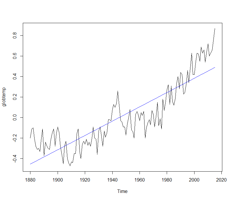
Both intercept and slope coefficients are reported as significative. Let us plot the time series against the fit.
plot(globtemp)
lines(ts(fitted(trend_fit), start=1880, frequency = 1), col = 4)
We go on with the search for structural changes.
globtemp_brk <- breakpoints(globtemp ~ tt, h = 0.1)
summary(globtemp_brk)
	 Optimal (m+1)-segment partition:

Call:
breakpoints.formula(formula = globtemp ~ tt, h = 0.1)

Breakpoints at observation number:

m = 1                  84
m = 2      23          84
m = 3      27       66 84
m = 4      23    53 66 84
m = 5   16 32    53 66 84
m = 6   16 32    53 66 84 97
m = 7   16 32    53 66 84 97     117
m = 8   16 32    53 66 84 97 110 123
m = 9   14 27 40 53 66 84 97 110 123

Corresponding to breakdates:

m = 1                            1963
m = 2        1902                1963
m = 3        1906           1945 1963
m = 4        1902      1932 1945 1963
m = 5   1895 1911      1932 1945 1963
m = 6   1895 1911      1932 1945 1963 1976
m = 7   1895 1911      1932 1945 1963 1976      1996
m = 8   1895 1911      1932 1945 1963 1976 1989 2002
m = 9   1893 1906 1919 1932 1945 1963 1976 1989 2002

Fit:

m   0         1         2         3         4         5         6         7         8         9
RSS    3.3697    1.6670    1.2446    1.0202    0.8907    0.8229    0.7975    0.7739    0.7889    0.8282
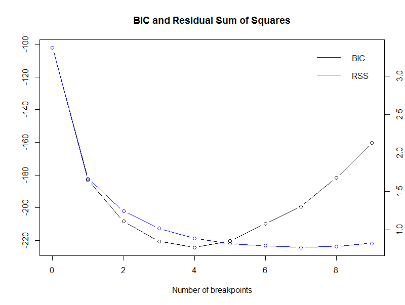
BIC -102.2140 -183.1946 -208.1954 -220.4943 -224.2281 -220.2494 -209.7707 -199.1243 -181.7788 -160.4341
plot(globtemp_brk)
The BIC minimum value is reached for m = 4.
plot(globtemp)
lines(fitted(globtemp_brk, breaks = 4), col = 4)
lines(confint(globtemp_brk, breaks = 4))
Break dates:
breakdates(globtemp_brk, breaks = 4)
[1] 1902 1932 1945 1963
Trend breaks coefficients:
coef(globtemp_brk, breaks = 4)
            (Intercept)           tt
1880 - 1902  -0.2312253 0.0008992095
1903 - 1932  -0.6037597 0.0084093437
1933 - 1945  -2.2475824 0.0374725275
1946 - 1963  -0.5640454 0.0070072239
1964 - 2015  -1.5983672 0.0173520874
Polinomial Fit Structural Changes
Second degree polinomial structural changes can be determined with the help of the following formula:
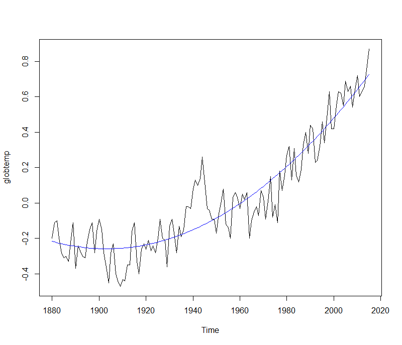
globtemp ~ tt + I(tt^2)
where tt is the globtemp timeline. Once again, we have first to verify that such regression makes sense for our time series by evaluating coefficients significance.
pol_fit <- lm(globtemp ~ tt + I(tt^2))
summary(pol_fit)
Call:
lm(formula = globtemp ~ tt + I(tt^2))

Residuals:
     Min       1Q   Median       3Q      Max
-0.27014 -0.08379  0.00685  0.07299  0.38625

Coefficients:
              Estimate Std. Error t value Pr(>|t|)
(Intercept) -2.124e-01  3.015e-02  -7.045 9.02e-11 ***
tt          -3.784e-03  1.016e-03  -3.725 0.000288 ***
I(tt^2)      7.860e-05  7.183e-06  10.943  < 2e-16 ***
---
Signif. codes:  0 ‘***’ 0.001 ‘**’ 0.01 ‘*’ 0.05 ‘.’ 0.1 ‘ ’ 1

Residual standard error: 0.1155 on 133 degrees of freedom
Multiple R-squared:  0.8696,	Adjusted R-squared:  0.8676
F-statistic: 443.3 on 2 and 133 DF,  p-value: < 2.2e-16
All coefficients are reported as significative. Let us plot the time series against the fit.
plot(globtemp, type = 'l')
lines(ts(fitted(pol_fit), start = 1880, frequency = 1), col = 4)
We go on with the search for structural changes.
globtemp_brk <- breakpoints(globtemp ~ tt + I(tt^2), data = globtemp, h = 0.1)
summary(globtemp_brk)
	 Optimal (m+1)-segment partition:

Call:
breakpoints.formula(formula = globtemp ~ tt + I(tt^2), h = 0.1,
    data = globtemp)

Breakpoints at observation number:

m = 1               66
m = 2   22          66
m = 3   22          66 84
m = 4   20 36       66 84
m = 5   20 36       66 84 97
m = 6   20 36    53 66 84 97
m = 7   20 36    53 66 84 97 112
m = 8   20 36    53 66 84 97 110 123
m = 9   19 32 45 58 71 84 97 110 123

Corresponding to breakdates:

m = 1                       1945
m = 2   1901                1945
m = 3   1901                1945 1963
m = 4   1899 1915           1945 1963
m = 5   1899 1915           1945 1963 1976
m = 6   1899 1915      1932 1945 1963 1976
m = 7   1899 1915      1932 1945 1963 1976 1991
m = 8   1899 1915      1932 1945 1963 1976 1989 2002
m = 9   1898 1911 1924 1937 1950 1963 1976 1989 2002

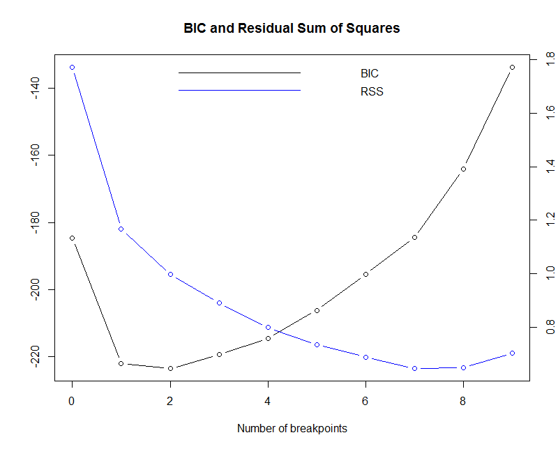
Fit:

m   0         1         2         3         4         5         6         7         8         9
RSS    1.7732    1.1662    0.9977    0.8903    0.7985    0.7348    0.6883    0.6453    0.6491    0.7024
BIC -184.6168 -221.9545 -223.5269 -219.3667 -214.5125 -206.1761 -195.4235 -184.5463 -164.0878 -133.7079
plot(globtemp_brk)
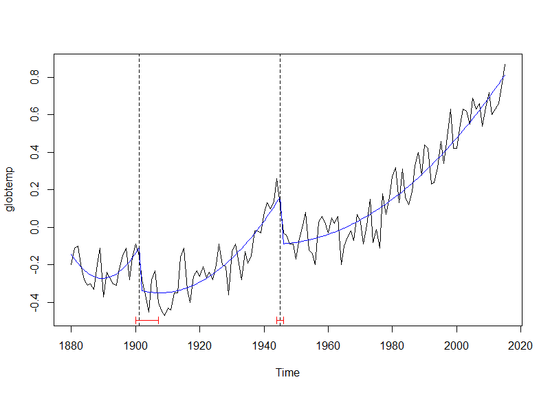
The BIC minimum value is reached for m = 2.
plot(globtemp)
lines(fitted(globtemp_brk, breaks = 2), col = 4)
lines(confint(globtemp_brk, breaks = 2))
Break dates:
breakdates(globtemp_brk, breaks = 2)
[1] 1901 1945
Polinomial fit breaks coefficients:
coef(globtemp_brk, breaks = 2)
           (Intercept)          tt      I(tt^2)
1880 - 1901 -0.11675325 -0.02862084 0.0013226990
1902 - 1945 -0.06025445 -0.02034837 0.0003589594
1946 - 2015  0.61164924 -0.02197550 0.0001724349
Auto-regressive Model Structural Changes
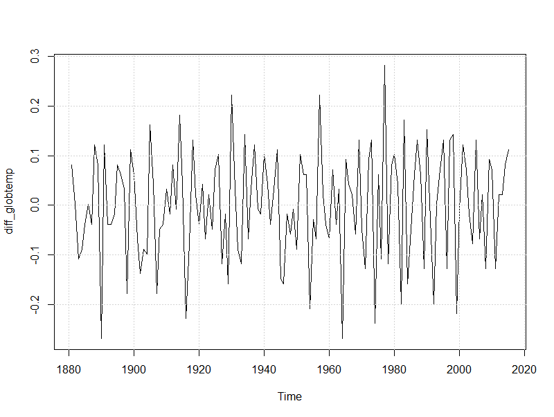
First differencing of the globtemp time series is computed to make it as stationary. The result is zero-centered by subtracting its mean.
diff_globtemp <- diff(globtemp) - mean(diff(globtemp))
plot(diff_globtemp, type = 'l')
grid()
The Augmented Dickey-Fuller test with type = “nc” having the following null hypothesis and test statistics is run.
$$
\begin{equation}
\begin{cases}
\ Model:\ \Delta y_{t}\ =\ \gamma y_{t-1} + \epsilon_{t} \\
\\
H_{0}: \gamma = 0\ \ \ \ \ test\ statistics: \tau_{1} \\
\\
\end{cases}
\end{equation}
$$
urdftest_lag = floor(12*(length(diff_globtemp)/100)^0.25) # long
urdfTest(diff_globtemp, lags = urdftest_lag, type = c("nc"), doplot = FALSE)
Title:
 Augmented Dickey-Fuller Unit Root Test

Test Results:

  Test regression none

  Call:
  lm(formula = z.diff ~ z.lag.1 - 1 + z.diff.lag)

  Residuals:
       Min       1Q   Median       3Q      Max
  -0.21075 -0.06373  0.00499  0.07173  0.18976

  Coefficients:
               Estimate Std. Error t value Pr(>|t|)
  z.lag.1      -2.69424    0.69716  -3.865 0.000189 ***
  z.diff.lag1   1.35360    0.67167   2.015 0.046336 *
  z.diff.lag2   0.98047    0.64080   1.530 0.128899
  z.diff.lag3   0.69130    0.60389   1.145 0.254820
  z.diff.lag4   0.64252    0.56115   1.145 0.254718
  z.diff.lag5   0.47524    0.51691   0.919 0.359925
  z.diff.lag6   0.34398    0.46422   0.741 0.460287
  z.diff.lag7   0.26961    0.40719   0.662 0.509299
  z.diff.lag8   0.29206    0.34707   0.842 0.401906
  z.diff.lag9   0.20160    0.28928   0.697 0.487350
  z.diff.lag10  0.25317    0.22206   1.140 0.256761
  z.diff.lag11  0.17314    0.15559   1.113 0.268243
  z.diff.lag12  0.10922    0.09352   1.168 0.245440
  ---
  Signif. codes:  0 ‘***’ 0.001 ‘**’ 0.01 ‘*’ 0.05 ‘.’ 0.1 ‘ ’ 1

  Residual standard error: 0.1003 on 109 degrees of freedom
  Multiple R-squared:  0.6922,	Adjusted R-squared:  0.6555
  F-statistic: 18.86 on 13 and 109 DF,  p-value: < 2.2e-16


  Value of test-statistic is: -3.8646

  Critical values for test statistics:
        1pct  5pct 10pct
  tau1 -2.58 -1.95 -1.62
By comparing the test statistics with the critical value at 5% significance level, we reject the unit root null-hypothesis. Further, we run the KPSS test with type = “mu” to test the null hypothesis of level stationarity.
urkpssTest(diff_globtemp, type = c("mu"), lags = c("long"),  doplot = FALSE)
Title:
 KPSS Unit Root Test

Test Results:

  Test is of type: mu with 12 lags.

  Value of test-statistic is: 0.3308

  Critical value for a significance level of:
                  10pct  5pct 2.5pct  1pct
  critical values 0.347 0.463  0.574 0.739
Based on the reported test statistics and critical values, we cannot reject the null hypothesis of level stationarity. We then evaluate a linear regression model having lag-1 and lag-2 as regressor to fit the current value.
lag_1 <- lag(diff_globtemp, -1)
lag_2 <- lag(diff_globtemp, -2)
globtemp_df <- ts.intersect(dd0 = diff_globtemp, dd1 = lag_1, dd2 = lag_2)
summary(lm(dd0 ~ dd1 + dd2 - 1, data = globtemp_df))
Call:
lm(formula = dd0 ~ dd1 + dd2 - 1, data = globtemp_df)

Residuals:
      Min        1Q    Median        3Q       Max
-0.268417 -0.073502  0.007569  0.073164  0.266005

Coefficients:
    Estimate Std. Error t value Pr(>|t|)
dd1 -0.30442    0.08463  -3.597 0.000455 ***
dd2 -0.27040    0.08463  -3.195 0.001752 **
---
Signif. codes:  0 ‘***’ 0.001 ‘**’ 0.01 ‘*’ 0.05 ‘.’ 0.1 ‘ ’ 1

Residual standard error: 0.1029 on 131 degrees of freedom
Multiple R-squared:  0.1246,	Adjusted R-squared:  0.1112
F-statistic: 9.323 on 2 and 131 DF,  p-value: 0.0001639
Both lag-1 and lag-2 coefficients are reported as significant. Then we inspect if any structural change occurs for our auto-regressive model.
dd_brk <- breakpoints(dd0 ~ dd1 + dd2 - 1, data = globtemp_df, h = 0.1)
summary(dd_brk)
	 Optimal (m+1)-segment partition:

Call:
breakpoints.formula(formula = dd0 ~ dd1 + dd2 - 1, h = 0.1, data = globtemp_df)

Breakpoints at observation number:

m = 1                  78
m = 2                  78    102
m = 3               64 78    102
m = 4   19    36       78    102
m = 5   17    35    63 78    102
m = 6   17    35    63 78    102 120
m = 7   17    35 48 64 78    102 120
m = 8   17    35 48 64 78 93 106 119
m = 9   13 26 39 54 67 80 93 106 119

Corresponding to breakdates:

m = 1                            1960
m = 2                            1960      1984
m = 3                       1946 1960      1984
m = 4   1901      1918           1960      1984
m = 5   1899      1917      1945 1960      1984
m = 6   1899      1917      1945 1960      1984 2002
m = 7   1899      1917 1930 1946 1960      1984 2002
m = 8   1899      1917 1930 1946 1960 1975 1988 2001
m = 9   1895 1908 1921 1936 1949 1962 1975 1988 2001

Fit:

m   0        1        2        3        4        5        6        7        8        9
RSS    1.387    1.338    1.290    1.270    1.250    1.223    1.212    1.202    1.198    1.221
BIC -214.826 -204.918 -195.122 -182.486 -169.973 -158.211 -144.707 -131.090 -116.950  -99.757
plot(dd_brk)
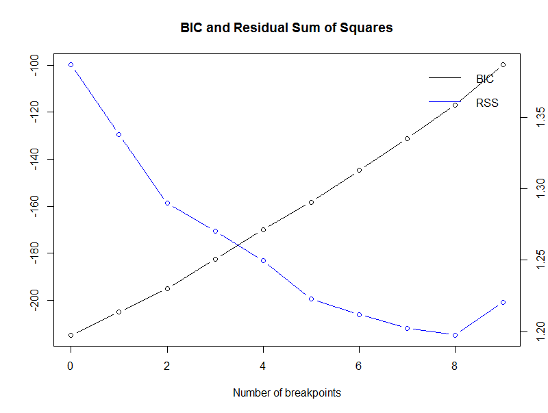
In this scenario, we cannot reach a conclusion for a value of m, as the BIC is minimum for m = 0. Ref. [1] shows a similar example and it points out that BIC was found to be somewhat unreliable for auto-regressive models by Bai and Perron. We then try to identify structural changes relying on a F statistics test available within the strucchange package as well.
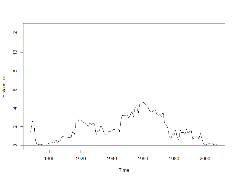
globtemp_Fstats <- Fstats(dd0 ~ dd1 + dd2 - 1, data = globtemp_df,  from = 0.05, to = 0.95)
plot(globtemp_Fstats)
No boundary crossing can be spotted (the boundary is represented by the red horizontal line on the top of the plot).
sctest(globtemp_Fstats, type = "supF")
	supF test

data:  globtemp_Fstats
sup.F = 4.7036, p-value = 0.7706
The sctest p-value confirms there is no significative breakpoint. We then conclude there are not any structural changes in the auto-regressive model under analysis.
Conclusions
After a basic exploration of the globtemp dataset, we leveraged on functions available within the strucchange package to date structural changes. Level, trend and second-degree polinomial fit breaks were identified. Differently, no breaks were found in the auto-regressive model based on lag-1 and lag-2 regressors. We further remark that the strucchange package provides with additional features such as generalized fluctuation tests as depicted by ref. [2].
If you have any questions, please feel free to comment below.
Disclaimer
- The present analysis is not intended to implement or to give basis for globtemp time series forecasts. It is intended for sake of introducing functionalities available within strucchange package.
References
-
[1] Applied Econometrics with R, Achim Zeileis, Christian Kleiber – Springer Ed.
[2] Strucchange package vignette
[3] Applied Econometrics Time Series, Walter Enders – Wiley Ed.
[4] GISS Surface Temperature Analysis (GISTEMP)
