A SIP application server (AS) text logs analysis may help in detection and, in some specific situations, prediction of different types of issues within a VoIP network. SIP server text logs contain the information which is difficult to obtain or even cannot be obtained from other sources, such as CDRs or signaling traffic captures.
The following parameters, among others, can help in estimating VoIP signaling network status:
- SIP dialog length. SIP dialog length of hundreds or even thousands messages points to a possible IP network problem, VoIP equipment malfunction, SIP signaling fraud, abnormal subscriber behavior
- Number and type of SIP messages retransmissions. A relatively high number of the retransmissions may be caused by AS hardware (HW) and/or software (SW) issues, IP network issues, peer SIP entities issues
- Request-response times for different SIP transactions in different SIP dialogs. Request-response time trends can help to predict overloads, IP network issues etc.
Depending on signaling load, a SIP AS can generate up to several tens of gigabytes of logs in text format per day, that’s why analysis of the SIP AS text logs is time- and resource-consuming task. Pandas data frames (DF) can help in such analysis. Pandas provides powerful tools for working with large DFs. Maximization of large DF processing speed may be achieved, in particular, by vectorizing all operations applied to the DF. Other techniques also may be used. All of the code for this article is available on GitHub.
SIP text log file processing steps:
- Open a SIP text log file for reading. I recommend opening SIP text log files in the same order as they were created by AS SW
- Read one line at a time from the opened SIP log file
- Extract SIP messages. Usually, these messages are located between specific delimiters
- Create a list consisting of dictionaries. Each of the dictionaries consists of SIP message timestamp (key) and SIP messages (value, as a list)
- Save the list to a pickle file on HDD or network storage. The file will be used for creating different DFs
- Create a DF containing specific information extracted from SIP messages stored in the pickle file
In this concrete case, the SIP DF contains the following columns:
- ‘Timestamp’ – added by SIP AS
- ‘Call-ID’ – extracted from SIP ‘Call-ID’ header
- ‘CSeq_num’, ‘CSeq_meth’ – derived from CSeq header of a SIP message
- ‘Direction’ – transmitted (Tx->) or received (Rx<-) SIP message, added by SIP AS
- ‘SIP method’ – SIP method name
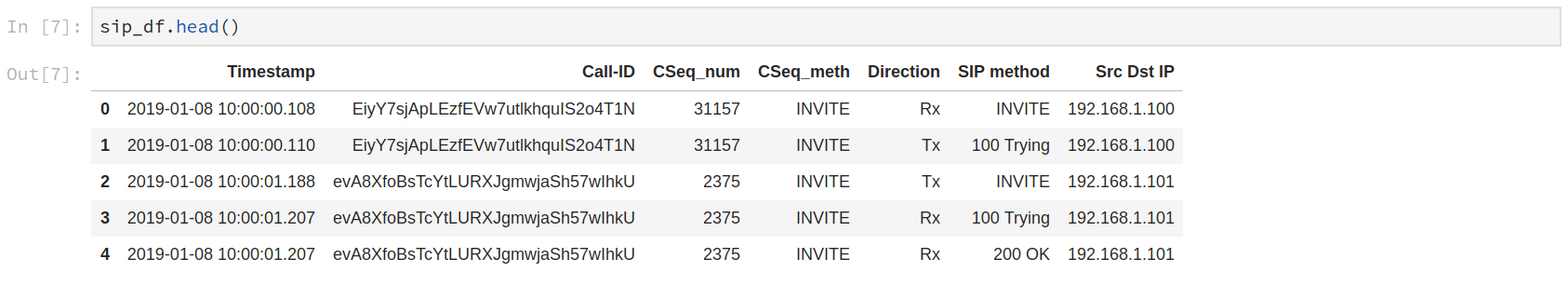
Fig. 1. SIP DF example
Having such SIP DF, we can extract some amount of helpful information. Count plots will be plotted using the following function:
def plot_data(df, col_name):
    fig, ax = plt.subplots(figsize=(20,6))
    ax.set(yscale = 'log')
    g = sns.countplot(x = col_name,  data = df, ax=ax)
    xticklabel = plt.setp(g.get_xticklabels(), rotation=90)
    plt.show()
DF sip_df will be used as a parameter for the functions described below.
1. SIP dialog length.
def sip_dialog_len(df):

    dfp = pd.pivot_table(df,index = ['Call-ID'], values = 'CSeq_num', aggfunc = 'count')\
    .sort_values(by = 'CSeq_num', ascending = False)
    dfp = dfp.rename(index=str, columns={"CSeq_num": "SIP dialog length"})
    return dfp
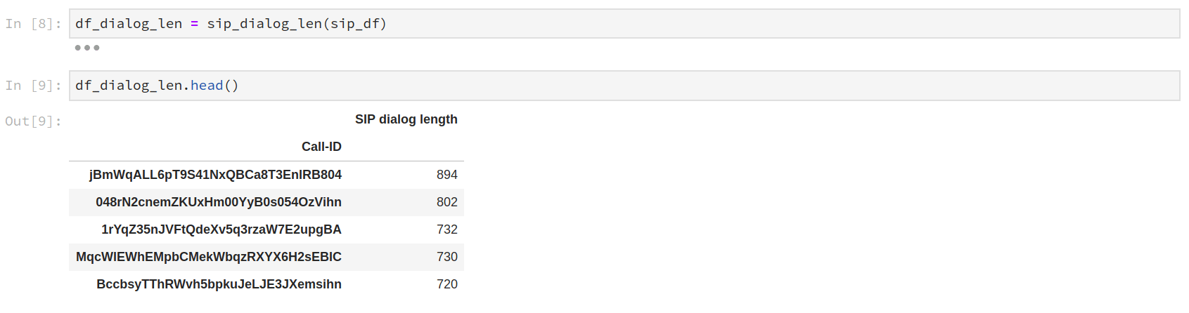
Fig. 2. The number of long SIP dialogs is very low, each dialog of length > 100 messages may be analysed for clarification the particular call scenario.
2. Request-response times (in ms) for transmitted INFO or INVITE requests
def req_resp_time_tx(df, transaction_type):

    # Remove retransmitted requests
    df = df.loc[df['SIP method'].shift() != df['SIP method']]

    # Add Req_Resp_Time column and fill it with 0 timedelta values
    df = df.assign(Req_Resp_Time = np.timedelta64(0, 'ms'))

    sip_method = transaction_type.split('-')[0]

    if sip_method in ['INFO', 'INVITE']:

        df['Req_Resp_Time'] = df[(((df['SIP method'] == sip_method) & (df['Direction'] == 'Tx')) |
                          ((df['SIP method'] == '200 OK') & (df['Direction'] == 'Rx')))].\
                                groupby(['Call-ID', 'CSeq_num', 'Src Dst IP'])['Timestamp'].diff()

        # Fill NaT cells
        df['Req_Resp_Time'].fillna(value = np.timedelta64(0, 'ms'), inplace = True)

        # Convert time diff to integer number of seconds
        df['Req_Resp_Time'] = df['Req_Resp_Time'].apply(lambda x: int(x / np.timedelta64(1, 'ms')))

        # Cut '000' from the end of timestamps, 'Timestamp' values converted to string
        df['Timestamp'] = df['Timestamp'].apply(lambda x: x.strftime('%H:%M:%S.%f'))
        df['Timestamp'] = df['Timestamp'].apply(lambda x: x[:-3])

        return df
    else:
        print('Incorrect transaction type!')
        return -1
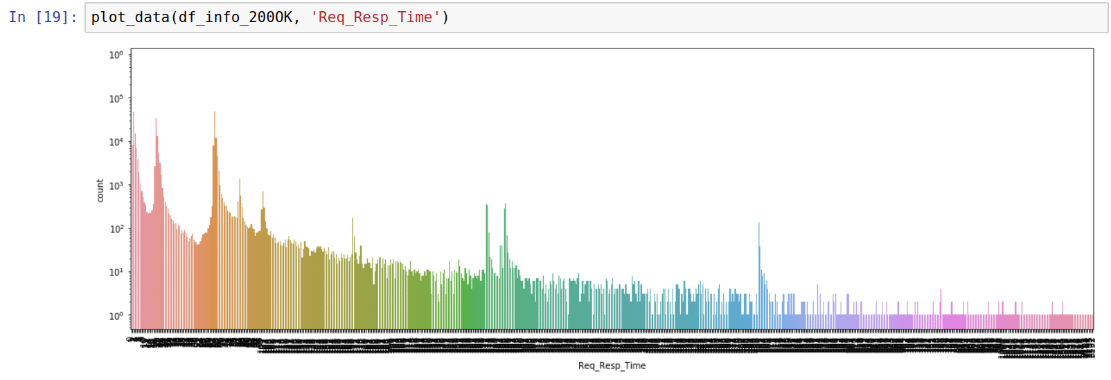
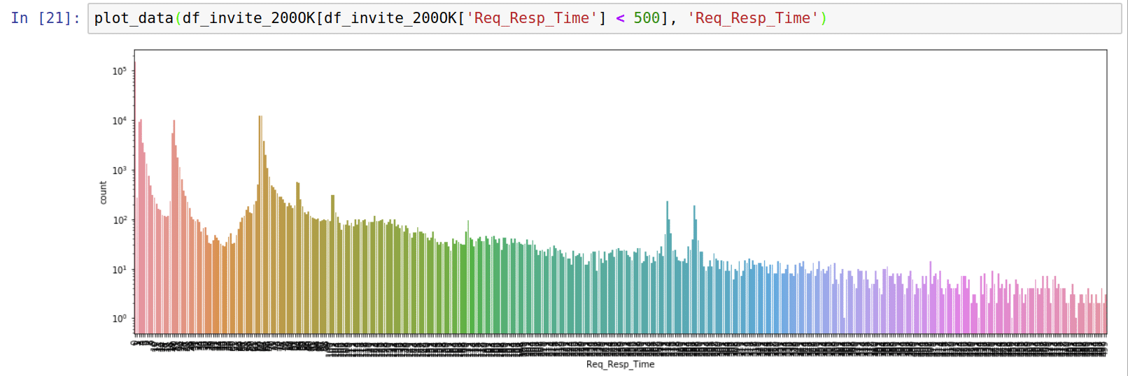
Fig. 3. Resp_Req_Time plots show approximately the same distribution of request-response times for INFO- and INVITE-transactions for the same groups of SIP peers. Request-response times > 500 ms point to retransmits. 500 ms is the default value for SIP T1 timer.
3. The number of retransmissions of INVITE or INFO requests.
Retransmit of a SIP request may be detected as a sequence of the transmitted SIP requests with the same Call-ID and SIP method and CSeq sequence number.
def retransmits_counter_tx(df, sip_method):

    dfx = df[(df['SIP method'] == sip_method) &
             (df['Direction'] == 'Tx')].\
              groupby(['Call-ID', 'CSeq_num']).count()
    df_rtr_tx = dfx[dfx['SIP method'] > 1]
    df_rtr_tx.reset_index(inplace = True)
    df_rtr_tx = df_rtr_tx.drop(['Timestamp', 'CSeq_meth',
                    'Direction', 'SIP method', 'Src Dst IP'], axis = 1)
    return df_rtr_tx
The function returns DF containing all the information necessary for further investigation of retransmission scenarios. Percentage of retransmissions of a SIP request:
def retransmissions_percentage(df_rtr, df):
    p = round(100 * df_rtr.shape[0]/df.shape[0], 2)
    return(str(p) + '%')
Example for INFO requests:
print(retransmissions_percentage(df_info_200OK_rtr, df_info_200OK))
0.1%
4. Request-response times (in ms) for received INFO-requests.
We cannot use Pandas groupby operation in this case because of the following reasons:
- Different INFO-200 OK transactions in a SIP dialog may share the same Call-ID and CSeq_num values
- INFO-requests and 200 OK-responses belonging to different dialogs may arrive in arbitrary moments of time and, consequently, will be stored in SIP DF in arbitrary order
- Retransmits of INFO-requests are possible, i.e. ‘SIP method’ column may contain sequences of retransmitted INFO-requests and 200 OK-responses
One of possible solutions is splitting DF into two separate data frames df_req and df_resp. ‘Timestamp’, ‘Call ID’, ‘CSeq_num’, ‘SIP method’ columns are the same for both DFs, ‘TS_req’ and ‘TS_resp’ are unique for df_req and df_resp. ‘Call ID’ and ‘CSeq_num’ columns are necessary for further analysis of particular INFO-200 OK transactions.
def rx_info_tx_200OK_rrt(df):
    dfw = df[((df['SIP method'] == 'INFO') &
         (df['Direction'] == 'Rx')) |
        ((df['SIP method'] == '200 OK') &
         (df['Direction'] == 'Tx'))][['Timestamp', 'Call-ID', 'CSeq_num', 'SIP method']]

    # Sorting is necessary since requests may be arbitrary mixed with responses
    dfw.sort_values(by = ['Call ID', 'CSeq_num'], inplace=True)

    # Add request and response timestamps columns
    dfw = dfw.assign(TS_Req = pd.NaT)
    dfw = dfw.assign(TS_Resp = pd.NaT)

    # Fill request timestamps columns with timestamps from Timestamps column
    dfw.at[dfw[dfw['SIP method'] == 'INFO'].index, 'TS_Req'] = \
           dfw['Timestamp'].loc[dfw[dfw['SIP method'] == 'INFO'].index]

    # Fill response timestamps column with timestamps from Timestamps column
    dfw.at[dfw[dfw['SIP method'] == '200 OK'].index, 'TS_Resp'] = \
           dfw['Timestamp'].loc[dfw[dfw['SIP method'] == '200 OK'].index]

    df_req = dfw[['Call-ID', 'CSeq_num', 'TS_Req']].dropna().reset_index()
    df_resp = dfw[['Call-ID', 'CSeq_num', 'TS_Resp']].dropna().reset_index()

    # Calculate request-response time difference
    df_req['Req_Resp_Time'] = df_resp['TS_Resp'] - df_req['TS_Req']

    df_req['Req_Resp_Time'] = df_req['Req_Resp_Time'].apply(lambda x: x/np.timedelta64(1, 'ms'))
    # Call-ID and CSeq_num will be necessary for searching specific scenario in
    # SIP AS log or in sip_df
    df_req = df_req[['Call-ID', 'CSeq_num', 'Req_Resp_Time']]

    return df_req
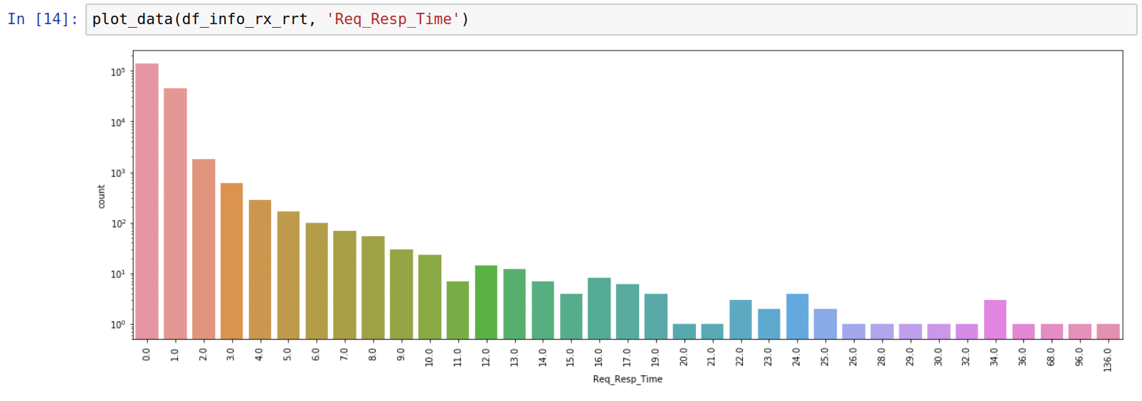
Fig. 4. Request-response time count plot for received INFO messages
Conclusion
Pandas DFs may be used as an additional tool for obtaining helpful information from SIP logs. Some of the methods described in this post may be used to analyze text log files of other protocols based on the request-response model.