In many business lines, it is more expensive to acquire new customers than to keep the ones they already have. So, businesses attempt to leverage historical customer behavior data to proactively understand customer segments who may likely leave the company for various reasons. This post is a follow-up to a previous article that focused on handling and working with categorical features as it relates to customer attrition analysis.
Motivation
Analytical challenges in multivariate data analysis, predictive modeling & prescriptive analytics include identifying redundant and irrelevant features. A recommended approach is to first address the redundancy; which can be achieved by identifying groups of input features that are as correlated as possible among themselves and as uncorrelated as possible with other variable groups in the same data set. On the other hand, relevancy is about potential predictor features and involves understanding the relationship between the target variable and input features. The current post illustrates two data analytics examples of reducing the number of categorical features in a data set to only the most useful features for predictive modeling & prescriptive analytics of customer churn. The first section illustrates multiple correspondence analysis using the prince library and the second section is related to best subset selection tool using chi-squared statistical test for categorical features from the scikit-learn library.
Multiple correspondence analysis is a multivariate data analysis and data mining tool concerned with interrelationships amongst categorical features. For categorical feature selection, the scikit-learn library offers a selectKBest class to select the best k-number of features using chi-squared stats (chi2). Such data analytics approaches may lead to simpler predictive models that can generalize customer behavior better and help identify at-risk customer segments. Such prescriptive analytics efforts may also help identify customer segments that may likely respond to targeted messaging, customer loyalty promotions and retention incentives.
Load Required Libraries
import pandas as pd
import matplotlib.pyplot as plt
import seaborn as sns
import prince # for multiple correspondence analysis
from sklearn.feature_selection import SelectKBest, chi2 # for chi-squared feature selection
from sklearn.preprocessing import LabelEncoder, OrdinalEncoder
Import and Prepare Dataset for Analysis
The Customer churn data set used in this post was obtained from this site. It’s a telecom company data that included customer-level demographic, account and payment services information, among others. Customers who left the company for competitors (Yes) or staying with the company (No) have been identified in the last column labeled Churn.
churn1 = pd,read_csv(‘C://Users// path to the location of your copy of the saved customer churn csv data file //Customer_churn.csv')
For brevity, I have included python code snippet (without code comments) shown below that I used to process the customer churn data set for exploratory data analysis previously. You may want to refer to the previous post for the steps used and the rational in preparing and handling the imported customer churn data set.
senior = {0 : 'No',
        1 : 'Yes'}

churn1['SeniorCitizen'].replace(senior, inplace=True)

def tenure(data):
    if 0 < data  <= 24 :
        return 'Short'
    else:
        return 'Long'

churn1['tenure'] = churn1['tenure'].apply(tenure)

def charges(data):
    if 0 < data  <= 70 :
        return 'LowCharge'
    else:
        return 'HighCharge'

churn1['MonthlyCharges'] = churn1['MonthlyCharges'].apply(charges)
recode = {'No phone service' : 'No',
          'No internet service' : 'No',
            'Fiber optic' : 'Fberoptic',
            'Month-to-month' : 'MtM',
            'Two year' : 'TwoYr',
            'One year' : 'OneYr' ,
            'Electronic check' : 'check',
            'Mailed check' : 'check',
            'Bank transfer (automatic)' : 'automatic',
            'Credit card (automatic)' : 'automatic'
            }

churn1.replace(recode, inplace=True)
# drop customer ID  using pandass
churn1.drop(['customerID', 'TotalCharges'], axis=1, inplace=True)
Once the data set has been loaded in memory and you have successfully run the above python codes, you are ready to check for the structure of the pre-processed data set.
print("The original data set contains: {} rows and {} columns".format(churn1.shape[0], churn1.shape[1]))
print("Features of the original data set:\n", list(churn1.columns))

The original data set contains: 7043 rows and 19 columns
Features of the original data set:
 ['gender', 'SeniorCitizen', 'Partner', 'Dependents', 'tenure',
'PhoneService', 'MultipleLines', 'InternetService', 'OnlineSecurity',
'OnlineBackup', 'DeviceProtection', 'TechSupport', 'StreamingTV',
'StreamingMovies', 'Contract', 'PaperlessBilling',
'PaymentMethod', 'MonthlyCharges', 'Churn']
Next, you would want to check for the number of categorical features in the pre-processed data set.
# number of categorical features
print("Number of categorical features : {}".format(len(churn1.select_dtypes(include=['object']).columns)))
print("Number of continuous features : {}".format(len(churn1.select_dtypes(include=['int64', 'float64']).columns)))

Number of categorical features : 19
Number of continuous features : 0
How many data levels (unique data values) are there in each categorical feature?
churn1.nunique()
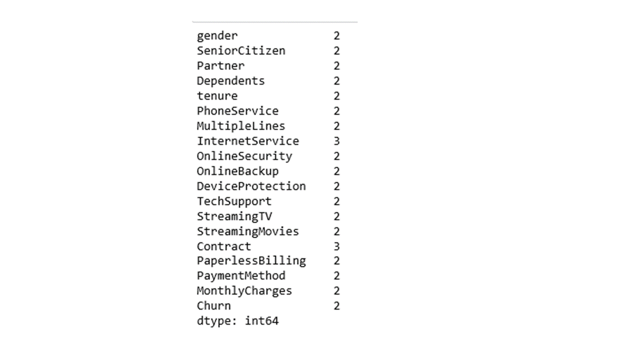
Looking at the code output above, most of the data fields contain two levels each, whereas InternetService & Contract columns are being coded with three levels each. Once we know the number of data levels in each field, the example codes below can be used to determine unique data values information within each data field.
churn1.Partner.value_counts()

No     3641
Yes    3402
Name: Partner, dtype: int64
Partner was coded as Yes and No; the corresponding numbers show row counts of each partner level in the data set.
churn1.InternetService.value_counts()

Fberoptic    3096
DSL          2421
No           1526
Name: InternetService, dtype: int64
InternetService has three levels as Fiberoptic InternetService, DSL InternetService or No InternetService.
churn1.Contract.value_counts()

MtM      3875
TwoYr    1695
OneYr    1473
Name: Contract, dtype: int64
Contract has three levels as MtM (month to month contract), TwoYr (two year contract) or OneYr (one year contract).
Multiple Correspondence Analysis
The python application of MCA using the prince library provides the option of constructing a low-dimensional visual representation of categorical variable associations.
The code below will initialize the MCA object to fit the churn data and will display MCA plot coordinates.
mca = prince.MCA(
        n_components=2,
        n_iter=3,
        copy=True,
        check_input=True,
        engine='auto',
        random_state=42
        )
churn_mca = mca.fit(churn1)

ax = churn_mca.plot_coordinates(
        X=churn1,
        ax=None,
        figsize=(8, 10),
        show_row_points=False,
        row_points_size=0,
        show_row_labels=False,
        show_column_points=True,
        column_points_size=30,
        show_column_labels=True,
        legend_n_cols=1
               ).legend(loc='center left', bbox_to_anchor=(1, 0.5))
Here is the MCA plot using the first two coordinates.
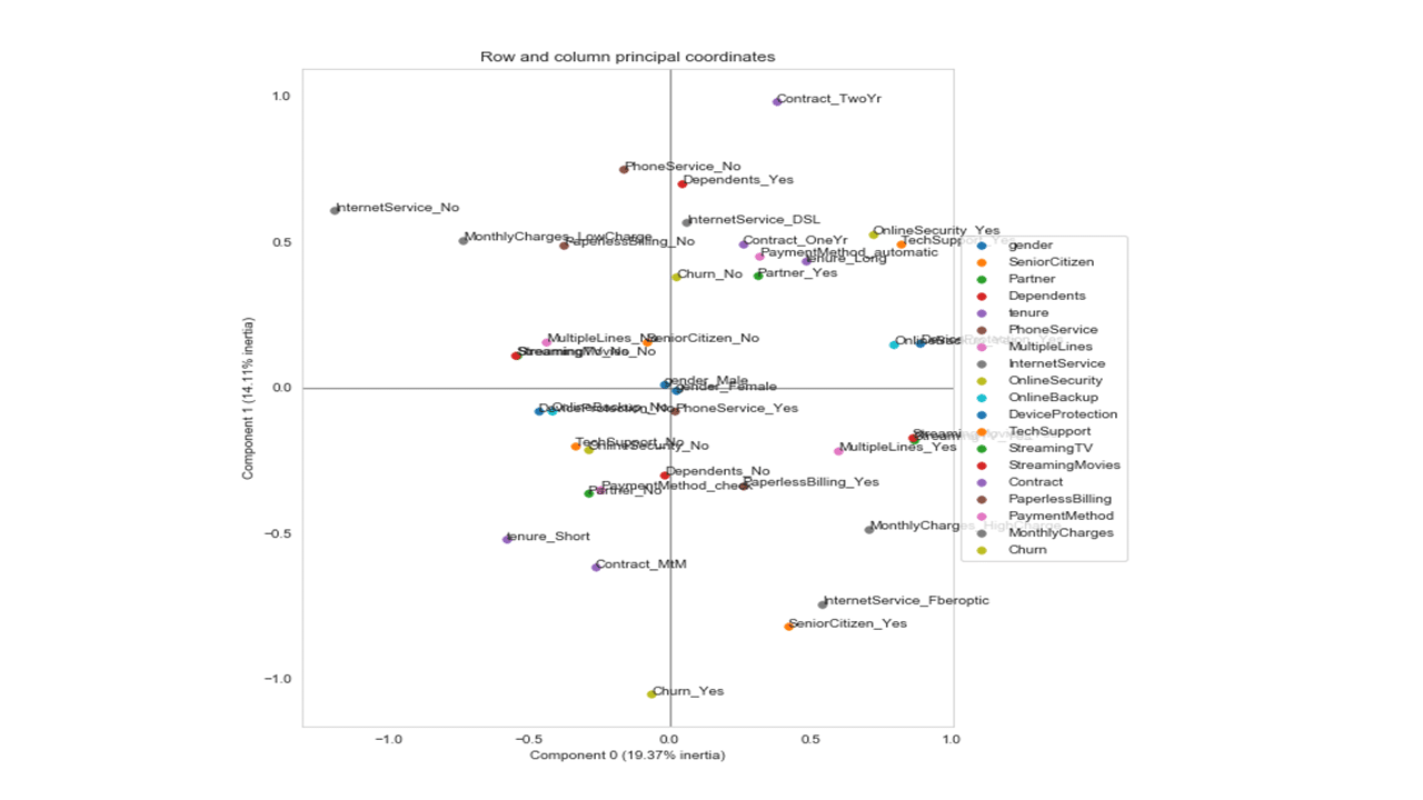
A general guide to interpreting the multiple correspondence analysis plot shown above for business insights would be to make a note as to how close input categorical features are to the target variable customer churn and to each other. For instance, senior citizens, customers with fiber optic internet service, those with month to month contractual agreements, and single customers or customers with no dependents are being related to a short tenure with the company and a propensity of high risk to churn. On the other hand, customers with more than a year contract, those with DSL internet service, younger customers, customers with multiple lines are being related to a long tenure with the company and a higher tendency to stay with company.
Best Subset Selection using the chi2 test stat for categorical features
Before you can employ selectKBest in the scikit-learn library, you need to coerce categorical features into indicator variables (dummy variables). There are many ways to creating dummy variables, two of which are; the get_dummies tool in pandas and OrdinalEncoder() / LabelEncoder() in the scikit-learn library.
get_dummies from the pandas library
The get_dummies algorithm available in the pandas library creates a DataFrame by coercing categorical features into one or more new features with values of 0 and 1.
churn2 = pd.get_dummies(churn1, drop_first=True)
Let’s Check data structure and data types of the transformed DataFrame.
print(churn2.shape)
print("The data set contains: {} rows and {} columns".format(churn2.shape[0], churn2.shape[1]))
print("Features after get_dummies:\n", list(churn2.columns))

(7043, 21)
The data set contains: 7043 rows and 21 columns
Features after get_dummies:
 ['gender_Male', 'SeniorCitizen_Yes', 'Partner_Yes', 'Dependents_Yes',
'tenure_Short', 'PhoneService_Yes', 'MultipleLines_Yes',
'InternetService_Fberoptic', 'InternetService_No',
'OnlineSecurity_Yes', 'OnlineBackup_Yes', 'DeviceProtection_Yes',
'TechSupport_Yes', 'StreamingTV_Yes', 'StreamingMovies_Yes',
'Contract_OneYr', 'Contract_TwoYr', 'PaperlessBilling_Yes',
'PaymentMethod_check', 'MonthlyCharges_LowCharge', 'Churn_Yes']
Next, you need to identify and specify columns representing the input features and the target variable using the code below.
X = churn2.drop('Churn_Yes', axis=1) # input categorical features
y = churn2['Churn_Yes'] # target variable
The data is now ready to run the selectKBest step with an option to request scores for ‘all’ or ‘k-number’ of categorical features.
The code shown below will produce scores and print the scores for each of the categorical features in the data set.
# categorical feature selection
sf = SelectKBest(chi2, k='all')
sf_fit = sf.fit(X, y)
# print feature scores
for i in range(len(sf_fit.scores_)):
    print(' %s: %f' % (X.columns[i], sf_fit.scores_[i]))
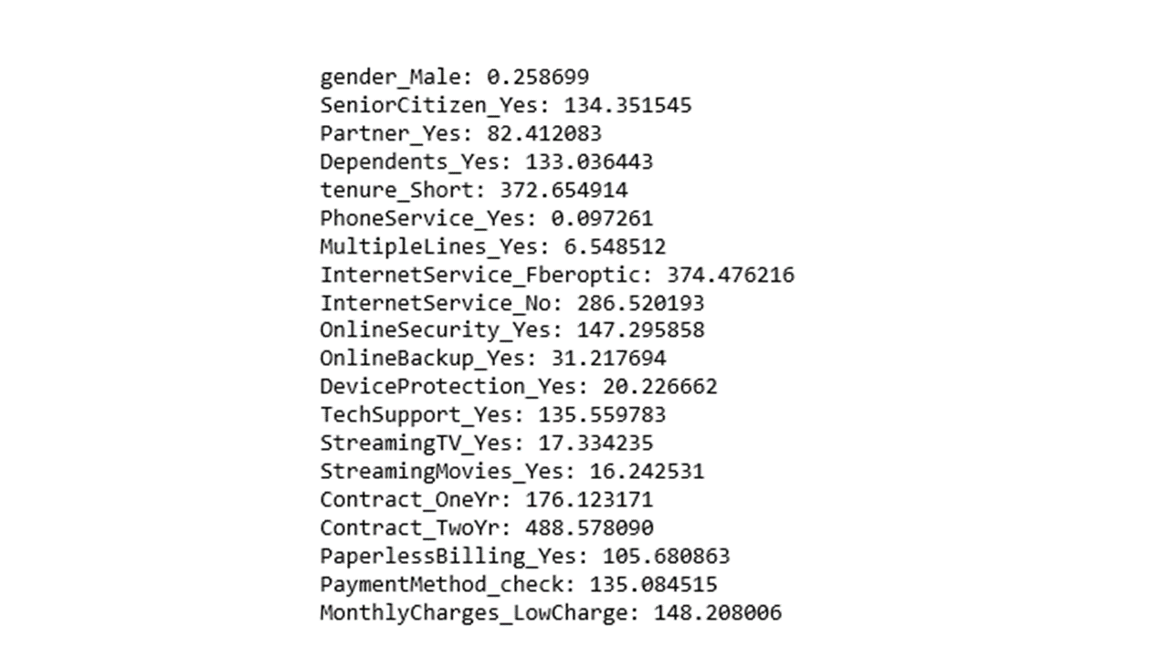
The way to interpret the above chi2 scores is that categorical features with the highest values for the chi-squared stat indicate higher relevance and importance in predicting customer churn and may be included in a predictive model development.
To aid for an easy selection of important categorical features, the following code will produce a visual display of the above scores sorted by the values from highest to lowest.
# plot the scores
datset = pd.DataFrame()
datset['feature'] = X.columns[ range(len(sf_fit.scores_))]
datset['scores'] = sf_fit.scores_
datset = datset.sort_values(by='scores', ascending=True)
sns.barplot(datset['scores'], datset['feature'], color='blue')
sns.set_style('whitegrid')
plt.ylabel('Categorical Feature', fontsize=18)
plt.xlabel('Score', fontsize=18)
plt.show()
Produces this plot.
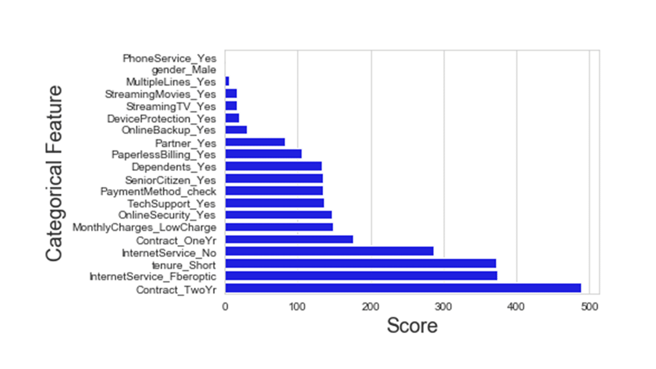
Looking at the chi2 scores and figure above, the top 10 categorical features to select for customer attrition prediction include Contract_TwoYr, InternetService_Fiberoptic, Tenure, InternetService_No, Contract_oneYr, MonthlyCharges, OnlineSecurity, TechSupport, PaymentMethod and SeniorCitizen.
Please note that the dummy-coding approach shown above was instrumental in selecting important feature-levels when the feature comprised more than two levels. The following approach is also being used to subset categorical features.
scikit-learn OrdinalEncoder() / LabelEncoder()
The OrdinalEncoder() and LabelEnocder() from the scikit-learn library can be used to encode each categorical feature to integers. First separate input features from target variable column using the code below.
X1 = churn1.drop('Churn', axis=1) # input features
y1 = churn1['Churn'] # target variable
Then, coerce categorical features into integers using the scikit-learn ordinal/label encoder
# prepare input features
oe = OrdinalEncoder()
oe.fit(X1)
X_enc = oe.transform(X1)

# prepare target variable
le = LabelEncoder()
le.fit(y1)
y_enc = le.transform(y1)
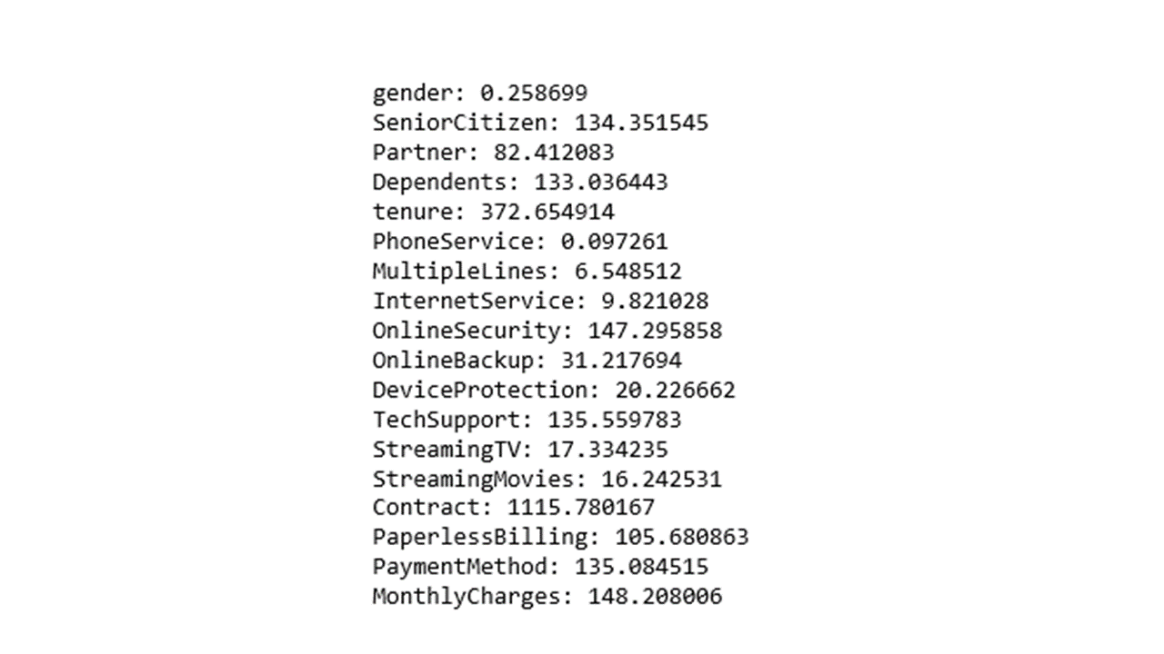
Subset (select) categorical features using the chi2 and plot the scores. To do these, the code shown below will produce and print scores for each categorical feature.
# feature selection
sf = SelectKBest(chi2, k='all')
sf_fit1 = sf.fit(X_enc, y_enc)
# print feature scores
for i in range(len(sf_fit1.scores_)):
    print(' %s: %f' % (X1.columns[i], sf_fit1.scores_[i]))
You could also plot the chi2 scores of categorical features using the code below.
# plot the scores of features
datset1 = pd.DataFrame()
datset1['feature'] = X1.columns[ range(len(sf_fit1.scores_))]
datset1['scores'] = sf_fit1.scores_
datset1 = datset1.sort_values(by='scores', ascending=True)
sns.barplot(datset1['scores'], datset1['feature'], color='green')
sns.set_style('whitegrid')
plt.ylabel('Categorical feature', fontsize=18)
plt.xlabel('Score', fontsize=18)
plt.show()
Produces this plot.
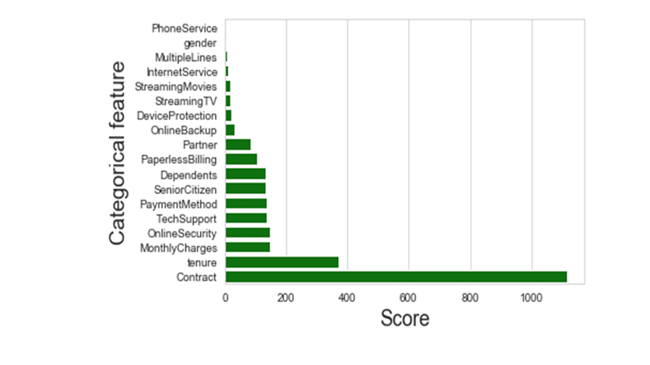
From the chi2 scores and the figure above, the top 10 categorical features to select for customer churn prediction include Contract, Tenure, MonthlyCharges, OnlineSecurity, TechSupport, PaymentMethod, SeniorCitizen, Dependents, PaperlessBilling and Partner.
In conclusion
This post attempted to illustrate two data analytics approaches that can be used to reduce the number of input categorical features in a data set and hence identify and select subsets of predictor features that are most relevant to predicting customer attrition. In the example data set, categorical features such as contract length, bill payment method, internet service type appeared to have played a role in customer attrition and retention. When selecting features in a real-world predictive modeling effort, analytics professionals and data scientists need to consult and work closely with domain experts and subject matter specialists. Besides, some machine learning (ML) algorithms will perform feature selection inherently, removing the necessity to do feature selection prior to running ML algorithms. The next step for this company would be to develop and deploy prescriptive & predictive models that would help identify better prospects & target existing customers with retention promotions and incentives addressing the propensity of risk to churn.