This is part 1 of a three-part article recently published in datasciene+. Part 1 illustrates the applications of python codes to programmatically download and parse a Wikipedia webpage into a dataset that is ready-to-use for subsequent data manipulation, processing, cleaning, crunching and advanced analytics. Part 2 and Part 3 dive right into the applications of two types of unsupervised machine learning algorithms using python.
Motivation
Data comes from disparate sources in all types, sizes, shapes, and in formats that are structured or unstructured. Social media, mobile, sensor or machine-generated data are some of the new data sources that hold the potential for data-driven value creation across diverse business lines and business segments. The web provides a rich source of data/information and presents ample opportunity to leverage unstructured and structured data sets to derive new insights. Hypertext Markup Language (HTML) is the most basic format of webpages. In general, HTML pages contain contents enclosed by several tags (words written within angle brackets), that instruct web browsers how to format the contents of the webpage per se. Python offers several tools and functions that can be of use to download, parse, manipulate and prepare data from several data types and formats including HTML into a ready-to-use form for data analysis. This publication contains examples of using such python libraries as Requests, BeautifulSoup, Pandas, Matplotlib and Seaborn for the downloading of online HTML content and data processing, cleaning, joining, and exploring datasets.
Load required libraries
import requests
from bs4 import BeautifulSoup
import time
import pandas as pd
import matplotlib.pyplot as plt
%matplotlib inline
import seaborn as sns
from sklearn.preprocessing import scale
The dataset
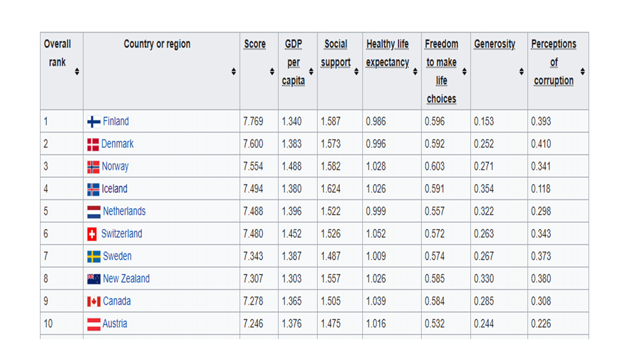
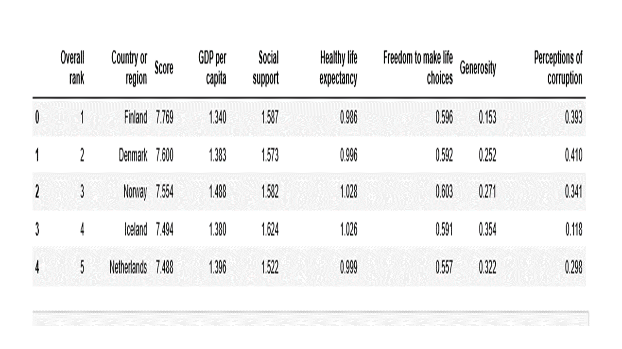
The HTML page for scraping in this post was published at this link. It is a world happiness report of 156 countries published by the United Nations on 20 March 2019. To give you a sense of what the report looks like, the image below shows the top 10 rows of the report.
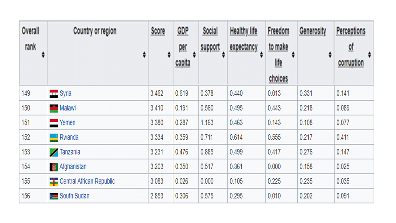
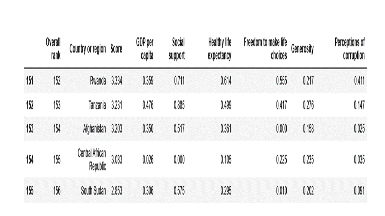
Below is an image of the last eight rows of countries in the report.
Retrieve the contents of a Wikipedia WebPage
The Requests library makes downloading online HTML content possible. To scrape the contents of the URL/webpage of interest, we need to invoke the requests.get function by specifying the URL/webpage for downloading. We then check for the response object of the request using the print() function as shown in the code below.
url = requests.get('https://en.wikipedia.org/wiki/World_Happiness_Report').text
time.sleep(1)
print(f"Response file type: {type(url)}")
print(f"The length of the response file is: {len(url)}")
print(f"Below are the first few lines of the response file: \n {url[:300]}")
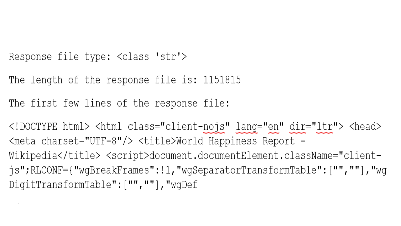
From the output above, our attempt to retrieve the contents of the webpage was successful. We now need a way to read and extract the information returned from the webpage. So, the BeautifulSoup library offers suitable parsers that can recognize HTML pages/tags and extract the contents contained in them.
Parsing the Contents of the WebPage
The next step is parsing the requests response object we saved above as a variable called url. For this step, we need to invoke the xml parser option in BeautifulSoup and create and save a Beautifulsoup object in a variable.
content = BeautifulSoup(url, "lxml")
Apply the print() function as the code below to reveal the text in the BeautifulSoup object.
print(content.text[7336:8000])
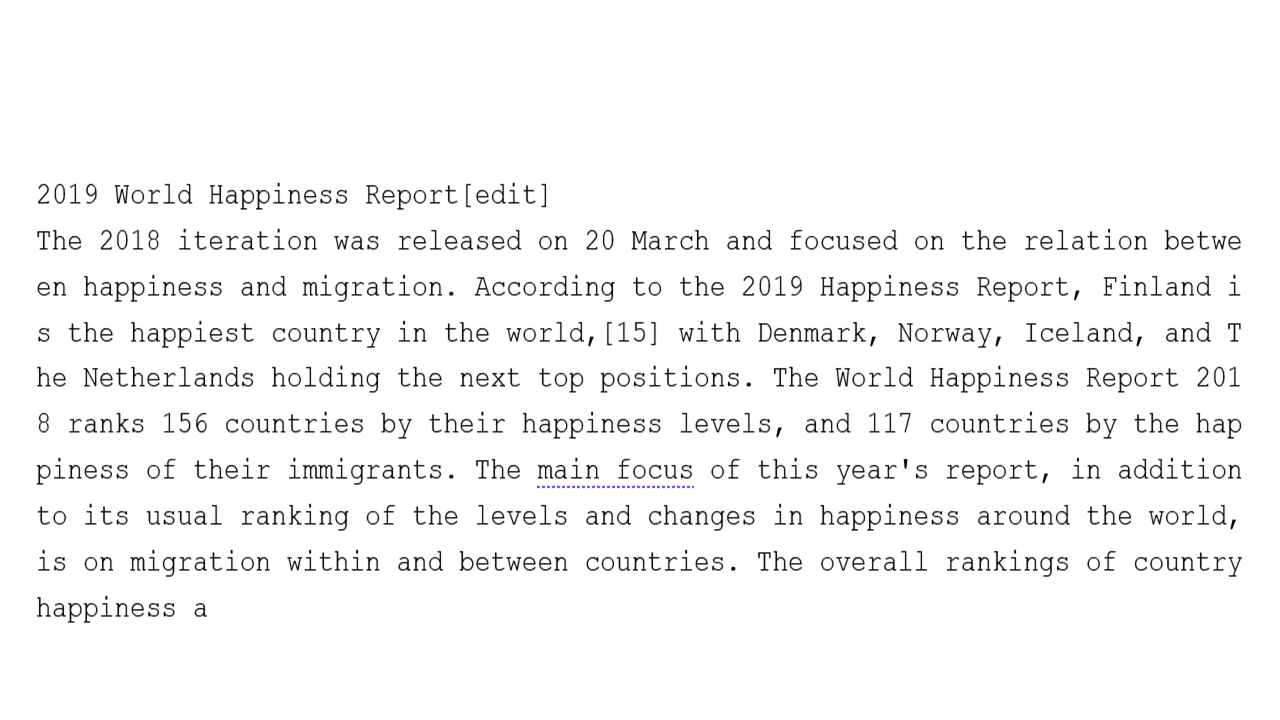
The output displayed above confirmed that we are on target regarding the contents of the webpage. The question now is how can we tell the unique identifier(s) that will allow us to parse the specific table/page of interest from within the BeautifulSoup object we just created? Well, parsing HTML entails identifying HTML elements and associated tags. So, the next step in this effort will be to launch the web browser and view the source HTML of the webpage and inspect the HTML format. When inspecting the page under the chrome browser inspector box, you will notice that the HTML section is a table class=“wikitable sortable jquery-table sorter” embedded within the tag ‘tr’.
We use the find() method to locate the HTML element table class=“wikitable sortable from within the BeautifulSoup object we saved above in a variable called content, followed by the select() method to zoom into the contents enclosed in the ‘tr’ tag. The output from running the code below is saved in variables My_table and My_table2.
My_table = content.find('table',{'class':'wikitable sortable'})
My_table2 = My_table.select('tr')
print(f"My_table is a: {type(My_table)}")
print(f"My_table2 is a: {type(My_table2)}")
print(f"The length of My_table2 is: {len(My_table2)}")
My_table is a:  class 'bs4.element.Tag'
My_table2 is a:  class 'list'
The length of My_table2 is: 157
Looking at the output above, My_table2 is a list of 157 elements. We use the print() function to reveal elements in My_table2. For instance, the code below prints out the first element of My_table2.
# reveal the first element
print(f"The first element in My_table2 contains:\n {My_table2[0]}")
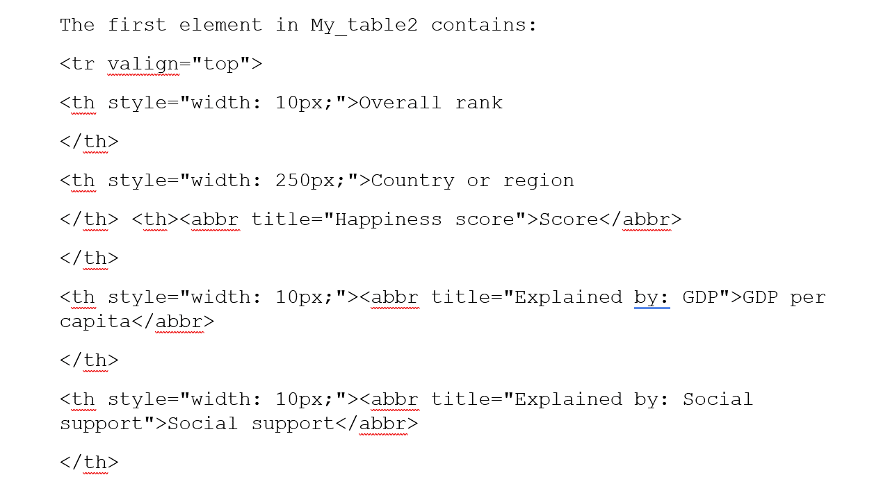
From the output above, the first element of My_table2 contained the nine column headings. The column headings were enclosed in tags ‘th’ nested in the tag ‘tr’.
We use the print() function to reveal the second element of My_table2.
# reveal the second element
print(f"The second element of My_table2 contains:\n {My_table2[1]}")
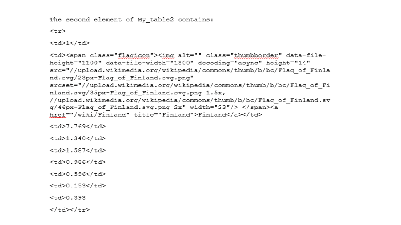
The second element of My_table2 contained data points for Finland that were enclosed in tags ‘td’ nested in the tag ‘tr’.
How about the last element of My_table2? Again, we use the print() function.
# reveal the last element of My_table2
print(f"The last element of My_table2 contains:\n {My_table2[156]}")
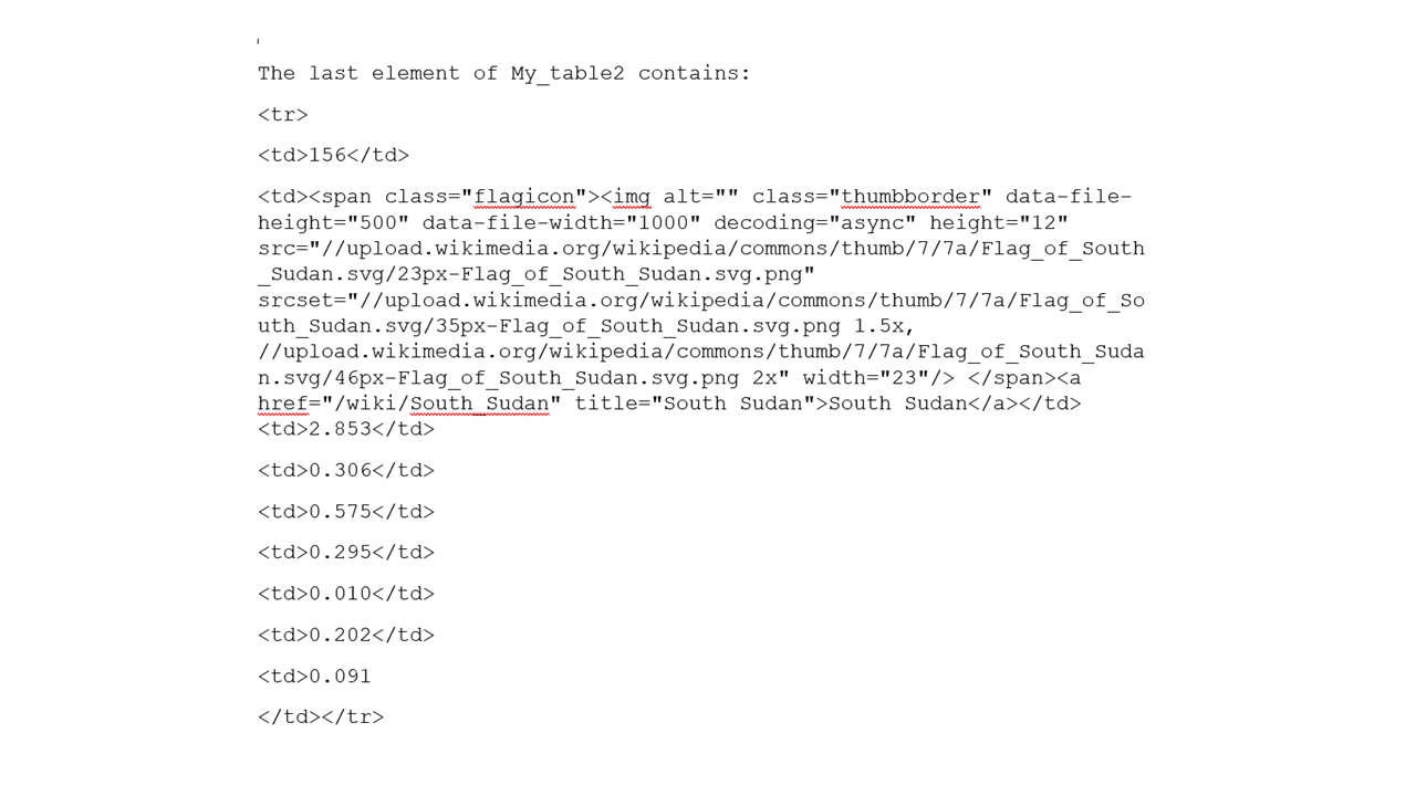
The last element of My_table2 contained data points for South Sudan that were enclosed in tags ‘td’ nested in the tag ‘tr’.
Now that we have information about the HTML structure that contained the specific web data, the steps below are aimed at parsing the HTML by making use of the select() method and iterating over the specific tags listed in the outputs above. The code below retrieves the column headings and the output text is saved in a variable called column_names.
column_names = []
for td in My_table2[0].select("th"):
    column_names.append(td.text.replace('\n', ' ').strip())
column_names
['Overall rank',
 'Country or region',
 'Score',
 'GDP per capita',
 'Social support',
 'Healthy life expectancy',
 'Freedom to make life choices',
 'Generosity',
 'Perceptions of corruption']
The code below iterates over the HTML to extract the rest of the data contained in My_table2 and creates lists of each data column. The individual lists will be appended to create a combined list.
tabcol1 = []
tabcol2 = []
tabcol3 = []
tabcol4 = []
tabcol5 = []
tabcol6 = []
tabcol7 = []
tabcol8 = []
tabcol9 = []

for tr in My_table2:
    dat = tr.select('td')
    if len(dat)==9:
        tabcol1.append(dat[0].find(text=True))
        tabcol2.append(dat[1].text.strip())
        tabcol3.append(dat[2].find(text=True))
        tabcol4.append(dat[3].find(text=True))
        tabcol5.append(dat[4].find(text=True))
        tabcol6.append(dat[5].find(text=True))
        tabcol7.append(dat[6].find(text=True))
        tabcol8.append(dat[7].find(text=True))
        tabcol9.append(dat[8].find(text=True))
Lastly, we create a dataframe by passing all the elements in the several lists above to a DataFrame() constructor.
Creating A DataFrame
df = pd.DataFrame(tabcol1,columns=[column_names[0]])
df[column_names[1]] = tabcol2
df[column_names[2]] = tabcol3
df[column_names[3]] = tabcol4
df[column_names[4]] = tabcol5
df[column_names[5]] = tabcol6
df[column_names[6]] = tabcol7
df[column_names[7]] = tabcol8
df[column_names[8]] = tabcol9

print(f"The table contains: {df.shape[0]} rows and {df.shape[1]} columns")
The dataframe contains: 156 rows and 9 columns
Data Exploration
Display the top rows of the dataframe.
df.head()
The first few rows look good. Similarly, display the last rows of the dataframe.
df.tail()
As seen from the row numbers and column headings, the dataframe contained 156 rows and 9 columns, as expected. We have successfully scraped the HTML page and prepared the data in a dataframe.
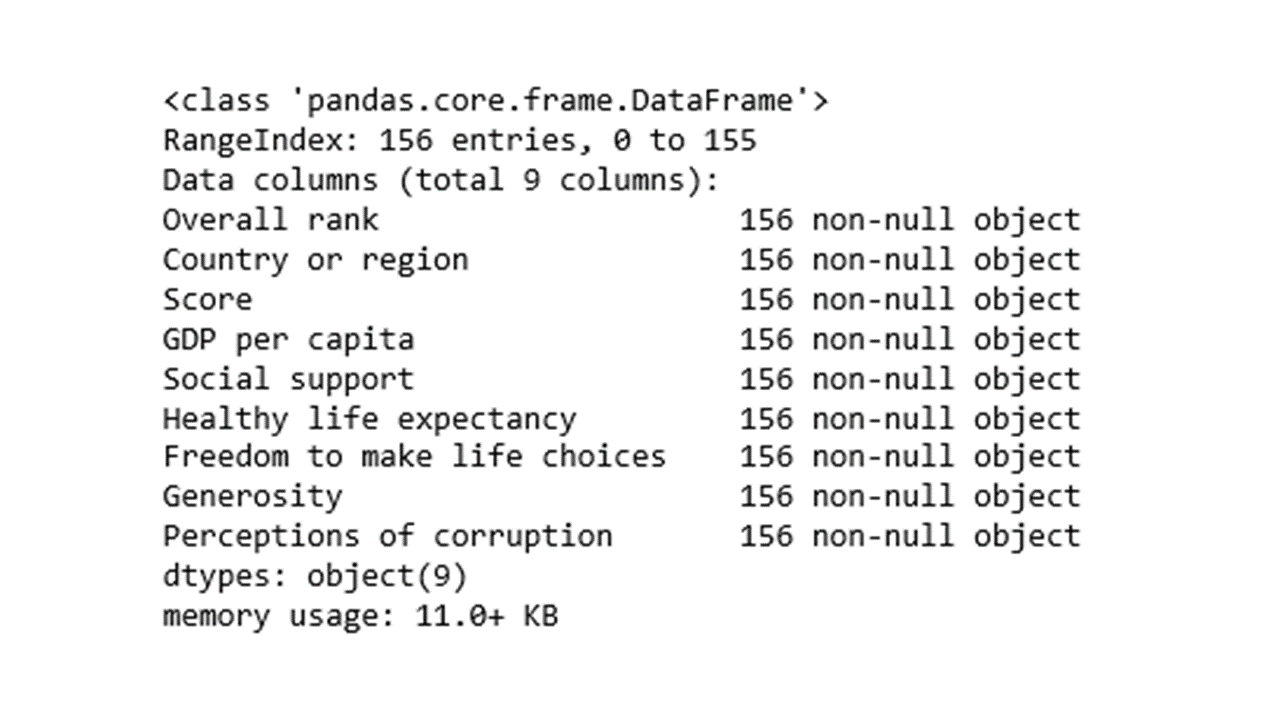
Gathering information about the different data fields is part of the early steps of data analysis.
df.info()
The column names may need some text cleaning. One easy way to clean messy column names could be achieved using the following code.
df.columns = df.columns.str.strip().str.lower().str.replace(' ', '_').str.replace('(', '').str.replace(')', '')
print(df.columns)
Index(['overall_rank', 'country_or_region', 'score', 'gdp_per_capita',
'social_support', 'healthy_life_expectancy', 'freedom_to_make_life_choices',
 'generosity', 'perceptions_of_corruption'], dtype='object')
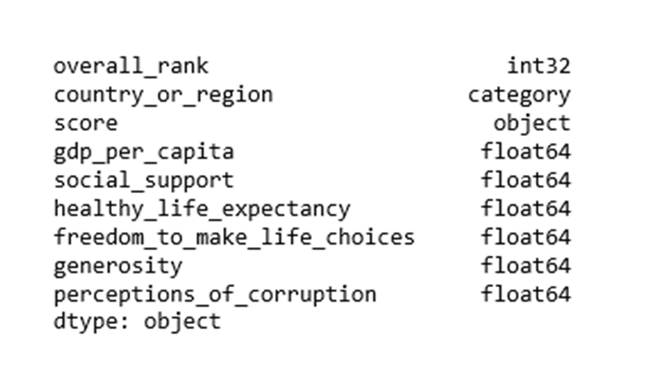
Coercing data types. The code below is to coerce many of the variables to numerical features and then check variable data types again.
numerical_features = ['gdp_per_capita', 'social_support', 'healthy_life_expectancy',
       'freedom_to_make_life_choices', 'generosity',  'perceptions_of_corruption']

df[numerical_features] = df[numerical_features].astype('float')

df['overall_rank'] = df['overall_rank'].astype('int')
df['country_or_region'] = df['country_or_region'].astype('category')
df.dtypes
Check for missing values in the dataset.
df.isnull().sum()
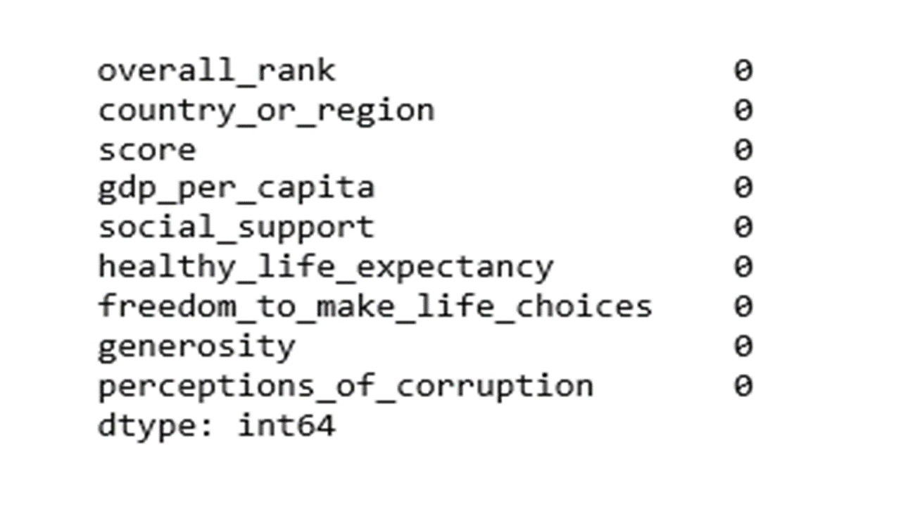
There are no missing values.
Writing the dataframe to a file: I will use the same dataset for an unsupervised machine learning topic covered in part 2 and part 3. The code below will write and save the dataset to a csv format.
df.to_csv('world_happiness_data19.csv', index=False)
Data visualization is an important tool for data exploration. Data distribution can be visually inspected using the box plot option. Box plots provide information about the variability of data and the extreme data values.
## prepare data for box plot
df2 = pd.melt(df, id_vars='country_or_region', value_vars=df[numerical_features])
plt.figure(figsize=(8,6))
sns.set(style="whitegrid")
sns.boxplot(y='variable',x='value', data=df2, palette="Set2")
plt.show()
Produces this figure!
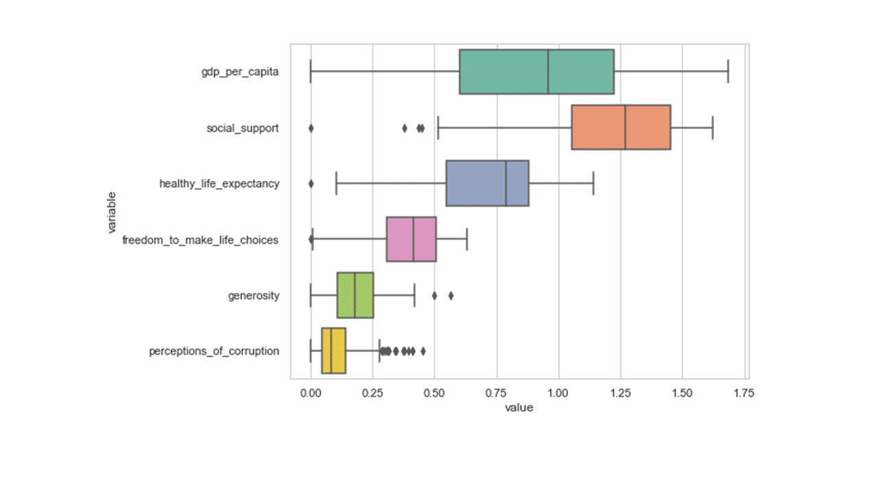
The middle 50% of the data, ranging from the 25th to the 75th percentile values, is being represented by the box.
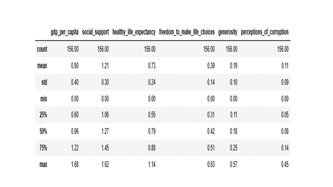
An easy way to create a descriptive summary stat in one go is the describe() function as shown in the code below.
df[numerical_features].describe().round(2)
The code below lists the top 10 countries based on the rank variable provided in the dataset.
print("Top 10 countries: \n {}".format((df[['overall_rank','country_or_region']][df['overall_rank']<=10]).to_string(index = False)))
Top 10 countries:
overall_rank country_or_region
1 Finland
2 Denmark
3 Norway
4 Iceland
5 Netherlands
6 Switzerland
7 Sweden
8 New Zealand
9 Canada
10 Austria
One other view of the dataset could be to group the 156 countries into say, five groups, based on the rank variable in the dataset. The code below will leverage pandas qcut() function to group the countries into quantiles of five groups and prints out the number of countries in each group. We may want to label the groups as Very Top Rank, Top Rank, Middle Rank, Low Rank, Very Low Rank.
df3 = pd.qcut(df['overall_rank'], 5,  labels=["Very Top Rank", "Top Rank", "Middle Rank", "Low Rank","Very Low Rank"])
df4 = pd.concat([df, df3], axis=1)
df4.columns=['overall_rank', 'country_or_region', 'score','gdp_per_capita', 'social_support', 'healthy_life_expectancy', 'freedom_to_make_life_choices', 'generosity',  'perceptions_of_corruption', 'group']
pd.value_counts(df4['group'])
Very Top Rank 32
Very Low Rank 31
Low Rank 31
Middle Rank 31
Top Rank 31
Name: group, dtype: int64
There are 32 countries in the first group and 31 countries assigned in each of the other four groups. When using the qcut() function, the number of countries in each of the five groups would have been equal had the total record count was divisible by 5.
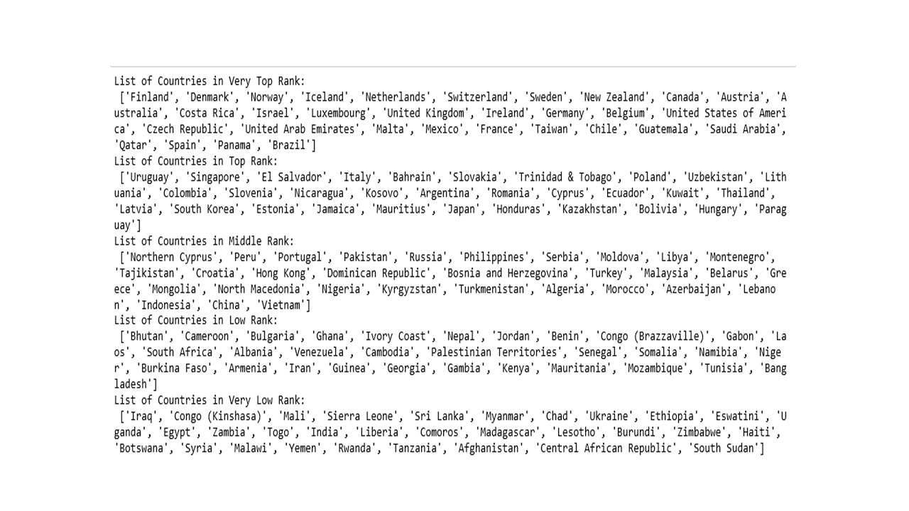
Now that countries have been assigned into five sub-groups, the code below lists country names by group.
for g in df4['group'].unique():
    tt = df4[['group','country_or_region']][df4['group']==g]
    print(f"List of Countries at {g}:  \n {list(tt['country_or_region'])}")
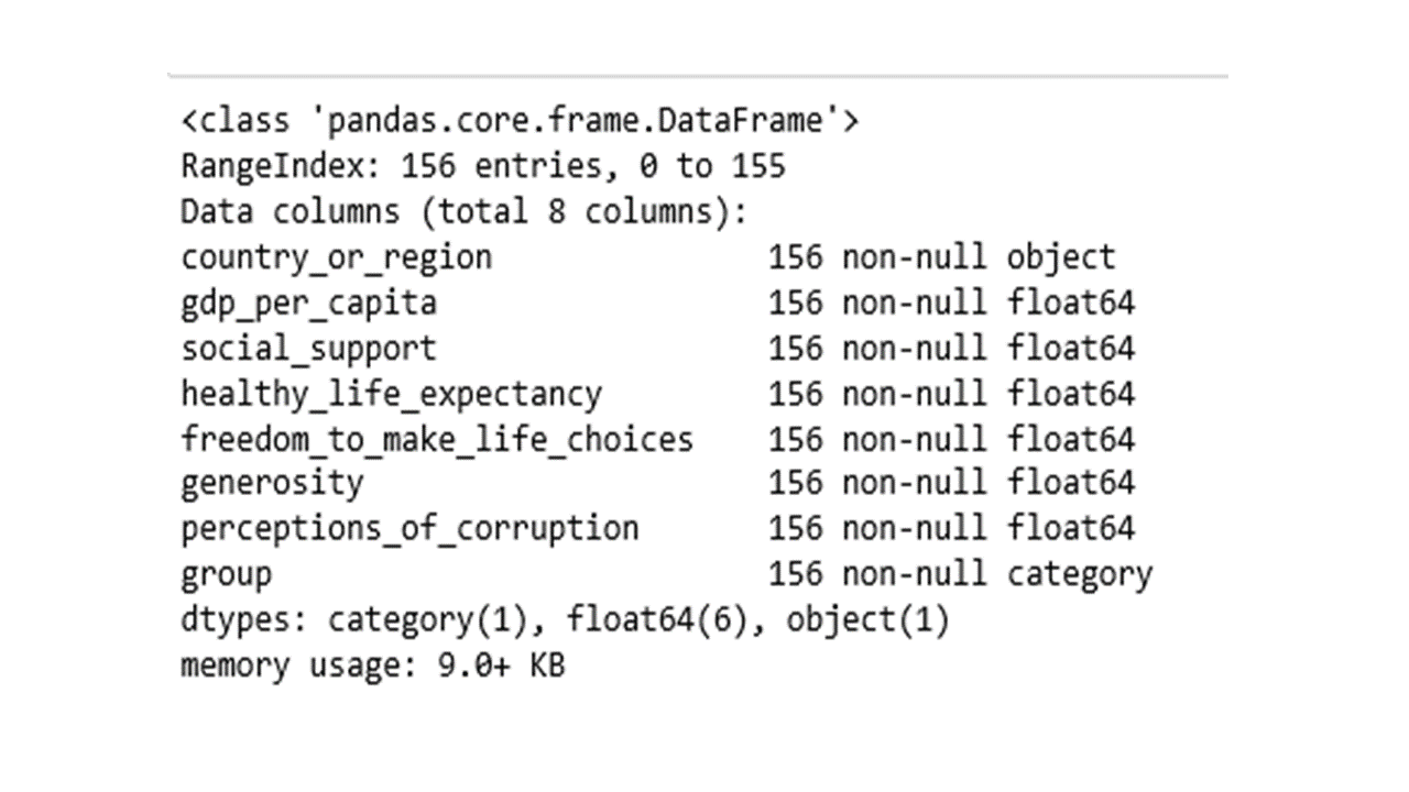
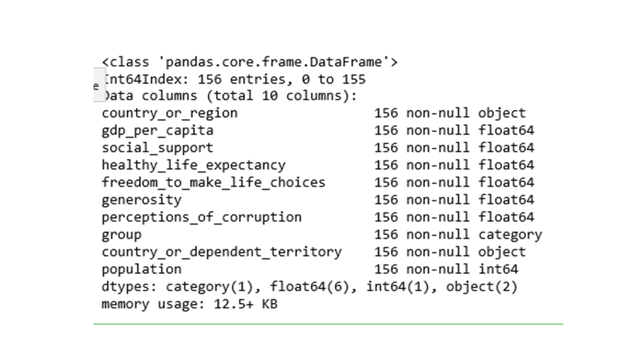
Sometimes it may be necessary to exclude variables from a dataset. The following code will drop two features related to the overall_rank and score from the dataframe.
df5 = df4.drop(['overall_rank','score'], axis=1)
df5.info()
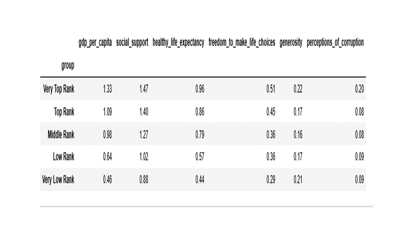
A handy way to inspect groups of countries is to leverage a ‘groupby’ object and compute group averages as in the code below.
tt1 = df5.groupby('group').mean().round(2)
tt1
A challenge exercise has been added below for you to write code following the steps/materials covered so far. Your to do list is below.
Adding a second data table challenge
The task is to scrape the Wikipedia page of the list of countries and dependencies by population (link provided below), and prepare a dataframe, and then merge the two dataframes using country as a ‘key’ to join them. You may consult the following steps when writing python code.
1) Write code to scrape the world population data published in this Wikipedia link
2) Create a dataframe that contains two columns related to country and population.
3) Remove duplicate records, if any.
4) Clean text regarding messy column names.
5) You will notice that some country names in the new dataset have additional notes and extra text, so you need to cleanup text of the country names by removing excess strings (notes and text), as well as trim excess white spaces, if present.
6) Coerce population variable to a numeric data type.
7) It is also a good idea to standardize country names in both data tables (change all country names in both dataframes to a lower case for example. Also see if country names are spelled the same way).
8) Once you have standardized/cleaned country names and column names, you may proceed to join the world population dataset with the happiness dataset from the exercise above.
Example python code related to the challenge exercise.
Scrape the Wikipedia list of countries and dependencies by population.
url = requests.get("https://simple.wikipedia.org/wiki/List_of_countries_and_dependencies_by_population").text
soup = BeautifulSoup(url, "lxml")
mytable =  soup.find('table',{'class':"wikitable sortable"})
mytable2 = mytable.select('tr')

colnames = []
for tr in mytable2[0].select('th'):
    colnames.append(tr.text.replace('\n','').strip())
colnames

tabcol1 = []
tabcol2 = []
tabcol3 = []
tabcol4 = []
tabcol5 = []
tabcol6 = []

for tr in mytable2:
    dat = tr.select('td')
    if len(dat)==6:
        tabcol1.append(dat[0].find(text=True))
        tabcol2.append(dat[1].text.strip())
        tabcol3.append(dat[2].find(text=True))
        tabcol4.append(dat[3].find(text=True))
        tabcol5.append(dat[4].find(text=True))
        tabcol6.append(dat[5].find(text=True))

new = pd.DataFrame(tabcol1,columns=[colnames[0]])
new[colnames[1]] = tabcol2
new[colnames[2]] = tabcol3
new[colnames[3]] = tabcol4
new[colnames[4]] = tabcol5
new[colnames[5]] = tabcol6

print(f"The table contains: {new.shape[0]} rows and {new.shape[1]} columns")
The table contains: 240 rows and 6 columns
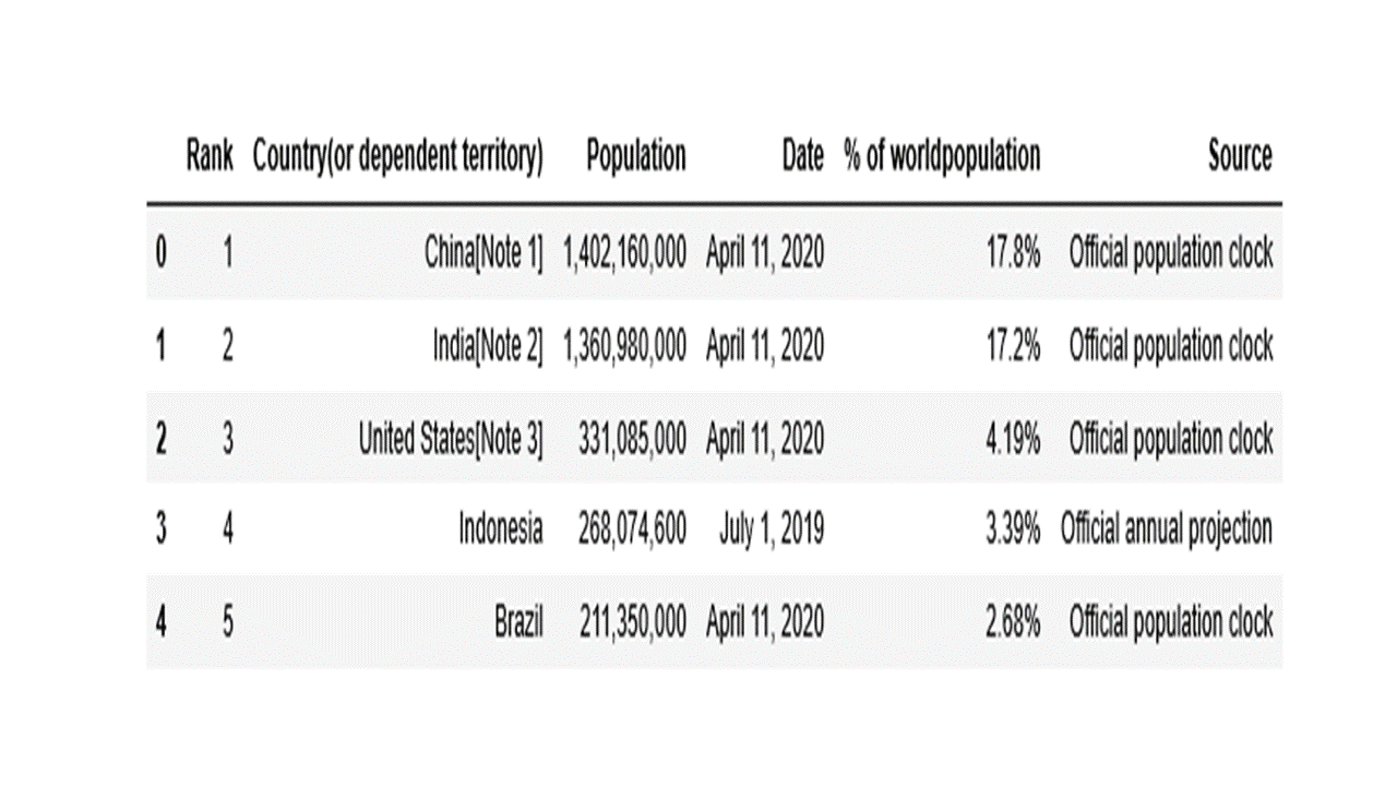
Check the top rows of the dataframe.
new.head()
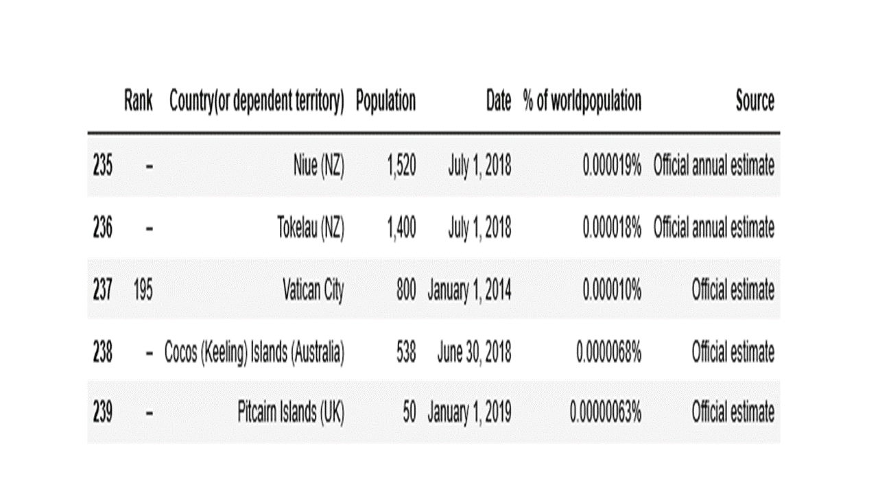
Inspect the last rows of the dataframe.
new.tail()
Clean messy column names.
new.columns = new.columns.str.lower().str.replace('(', ' ').str.replace(')', ' ').str.strip().str.replace(' ', '_')
print(new.columns)
Index(['rank', 'country_or_dependent_territory', 'population', 'date',
       '%_of_worldpopulation', 'source'],
      dtype='object')
Keep only country and population columns and then exclude duplicate records, if any.
new2 = new[['country_or_dependent_territory','population']]
new2.duplicated().sum()
0

There are no duplicate records.
Notice that some country names have additional notes and extra text, so you need to cleanup text by removing excess notes and text/strings. It is also a good idea to change country names to a lower case as well as remove excess white spaces, if present.
new2[['country_or_dependent_territory', 'extra','extra2']] = new2.country_or_dependent_territory.str.lower().str.strip().str.replace('(', '[').str.split("\[", expand=True,)
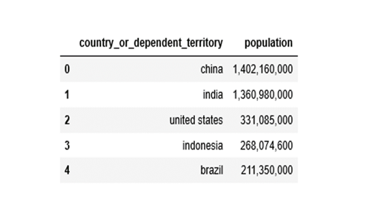
new3 = new2[['country_or_dependent_territory','population']]
new3.head()
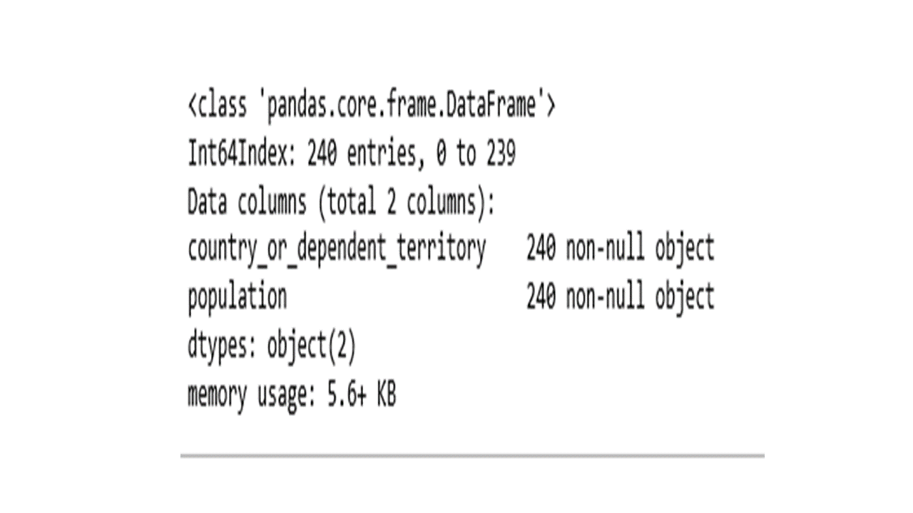
Check data types.
new2.info()
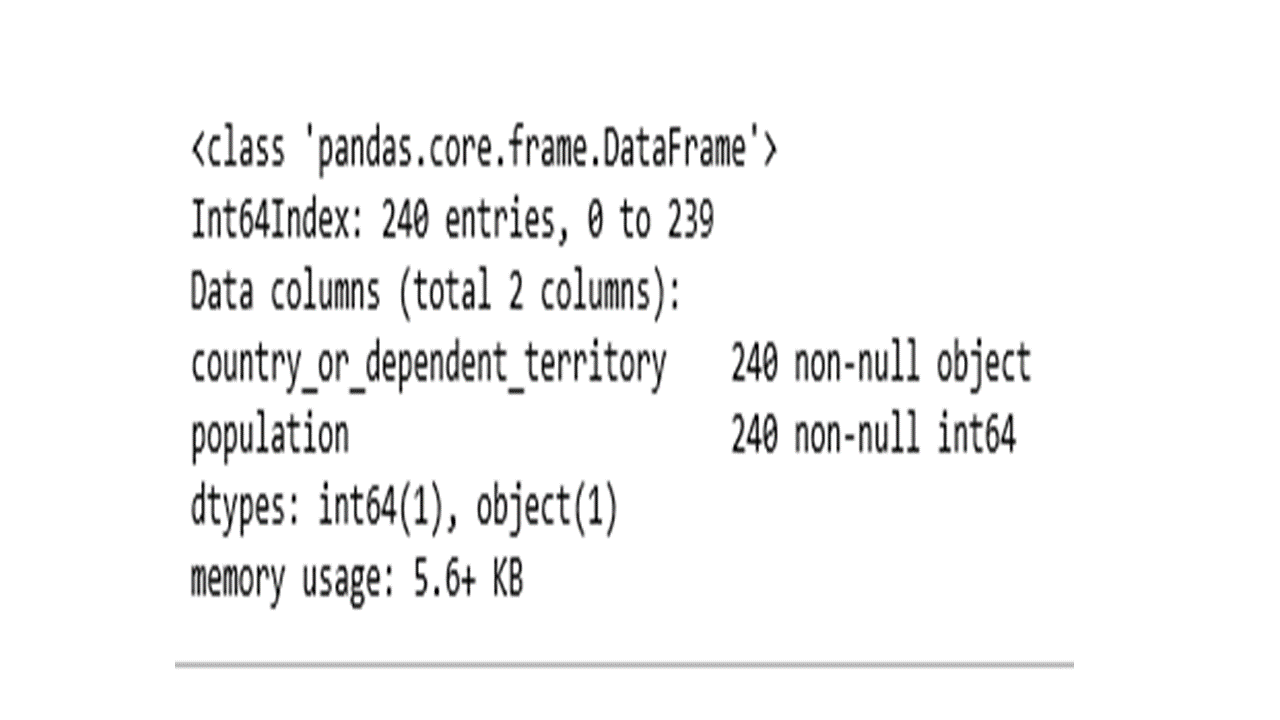
Coerce population column to a numeric variable.
new2['population'] = new2['population'].str.replace(',', '')
new2['population'] = pd.to_numeric(new2['population'], errors='coerce')
new2.drop(['extra','extra2'], axis=1, inplace=True)
new2.info()
Notice that some of the country names in the two data sets were not standardized. For instance, United States vs United States of America, Gambia vs The Gambia, Northern Cyprus vs Cyprus. The code below will recode selected country names, change country names to a lower case, as well as remove excess white spaces, if present.
# standardized country names via mapping
df5['country_or_region'] = df5['country_or_region'].str.lower().str.strip()
recode = {'united states of america' : 'united states',
          'trinidad & tobago' : 'trinidad and tobago',
           'palestinian territories' :'palestine' ,
           'congo (brazzaville)' : 'republic of the congo' ,
           'congo (kinshasa)' : 'democratic republic of the congo',
            'gambia' : 'the gambia',
           'northern cyprus' : 'cyprus',
           'hong kong' : 'hong kong '
            }


df5.replace(recode, inplace=True)
Merge the two datasets.
df_merged = pd.merge(df5, new2,  how='left', left_on=['country_or_region'], right_on=['country_or_dependent_territory'])
df_merged.info()
How many of the countries have missing population data?
df_merged[['country_or_region','population']].isna().sum()
country_or_region     0
population            0
dtype: int64
In Summary
An indispensable skill that aspiring data scientists need to cultivate is the ability to retrieve, integrate and manipulate the growing volumes of unstructured data with existing structured data, among others. Such skills are critical to answering more open-ended and complex business questions and delivering improved data insights. It is my hope that this post introduced you to python scripting that you might use in your next data analytics projects. Using the dataset prepared in this post, two companion posts published as Part 2 and Part 3 illustrate the applications of two unsupervised machine learning techniques.