Welcome to Part Two of the three-part tutorial series on proteomics data analysis. The ultimate goal of this exercise is to identify proteins whose abundance is different between a drug-resistant cell line and a control. That is we are looking for a list of differentially regulated proteins that may shed light on how cells escape the cancer-killing action of a drug. In Part One, I have demonstrated the steps to acquire a proteomics data set and perform data pre-processing. We will pick up from the cleaned data set and confront the missing value problem in proteomics.
Again, the outline for this tutorial series is as follows:
- Data acquisition and cleaning
- Data filtering and missing value imputation
- Statistical testing and data interpretation
Missing Value Problem
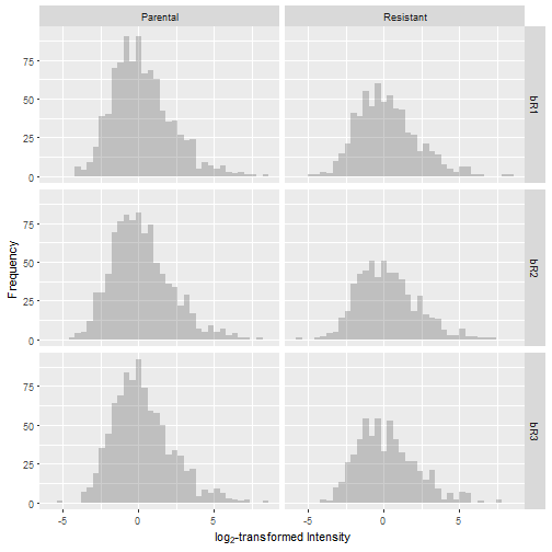
Although mass spectrometry-based proteomics has the advantage of detecting thousands of proteins from a single experiment, it faces certain challenges. One problem is the presence of missing values in proteomics data. To illustrate this, let's examine the first few rows of the log2-transformed and raw protein abundance values.
library(dplyr)   # for data manipulation

## View first 6 rows of the log2-transformed intensity
head(select(df, Gene, starts_with("LOG2")))
##    Gene LOG2.Parental_bR1 LOG2.Parental_bR2 LOG2.Parental_bR3
## 1 RBM47              -Inf              -Inf          21.87748
## 2 ESYT2           25.6019          25.56180          25.68763
## 3 ILVBL              -Inf          20.76474              -Inf
## 4 KLRG2              -Inf              -Inf          22.31786
## 5 CNOT1              -Inf              -Inf              -Inf
## 6   PGP              -Inf              -Inf              -Inf
##   LOG2.Resistant_bR1 LOG2.Resistant_bR2 LOG2.Resistant_bR3
## 1               -Inf               -Inf               -Inf
## 2               -Inf               -Inf               -Inf
## 3               -Inf               -Inf               -Inf
## 4               -Inf               -Inf               -Inf
## 5               -Inf               -Inf           29.14207
## 6               -Inf               -Inf           22.46269
## View first 6 rows of the raw intensity
head(select(df, Gene, starts_with("LFQ")))
##    Gene LFQ.intensity.Parental_bR1 LFQ.intensity.Parental_bR2
## 1 RBM47                          0                          0
## 2 ESYT2                   50926000                   49530000
## 3 ILVBL                          0                    1781600
## 4 KLRG2                          0                          0
## 5 CNOT1                          0                          0
## 6   PGP                          0                          0
##   LFQ.intensity.Parental_bR3 LFQ.intensity.Resistant_bR1
## 1                    3852800                           0
## 2                   54044000                           0
## 3                          0                           0
## 4                    5228100                           0
## 5                          0                           0
## 6                          0                           0
##   LFQ.intensity.Resistant_bR2 LFQ.intensity.Resistant_bR3
## 1                           0                           0
## 2                           0                           0
## 3                           0                           0
## 4                           0                           0
## 5                           0                   592430000
## 6                           0                     5780200
It is hard to miss the -Inf values, which represent protein intensity measurements of 0 in the raw data set. These data points have missing values, or a lack of quantification in the indicated samples. This is a common issue in proteomic experiments, and it arises due to sample complexity and variation (or stochasticity) in sampling from one run to another.
For example, imagine pouring out a bowl of Lucky Charms cereal containing a thousand different marshmallows. Let's say there is only one coveted rainbow marshmallow for every one thousand pieces. The likelihood of your bowl containing the rare shape is disappointingly low. In our situation, there are approximately 20,000 protein-coding genes in a given cell, and many in low quantities if expressed at all. Hence, the probability of consistently capturing proteins with low expression across all experiments is small.
Data Filtering
To overcome the missing value problem, we need to remove proteins that are sparsely quantified. The hypothesis is that a protein quantified in only one out of six samples offers insufficient grounds for comparison. In addition, the protein could have been mis-assigned.
One of many filtering schemes is to keep proteins that are quantified in at least two out of three replicates in one condition. To jog your memory, we have two conditions, one drug-resistant cell line and a control, and three replicates each. The significance of replicates will be discussed in Part 3 of the tutorial. For now, we will briefly clean the data frame and apply filtering.
## Data cleaning: Extract columns of interest
df = select(df, Protein, Gene, Protein.name, starts_with("LFQ"), starts_with("LOG2"))

## Display structure of df
glimpse(df)
## Observations: 1,747
## Variables: 15
## $ Protein                     <chr> "A0AV96", "A0FGR8", "A1L0T0", "A4D...
## $ Gene                        <chr> "RBM47", "ESYT2", "ILVBL", "KLRG2"...
## $ Protein.name                <chr> "RNA-binding protein 47", "Extende...
## $ LFQ.intensity.Parental_bR1  <dbl> 0, 50926000, 0, 0, 0, 0, 0, 0, 0, ...
## $ LFQ.intensity.Parental_bR2  <dbl> 0, 49530000, 1781600, 0, 0, 0, 0, ...
## $ LFQ.intensity.Parental_bR3  <dbl> 3852800, 54044000, 0, 5228100, 0, ...
## $ LFQ.intensity.Resistant_bR1 <dbl> 0, 0, 0, 0, 0, 0, 0, 0, 0, 8213400...
## $ LFQ.intensity.Resistant_bR2 <dbl> 0, 0, 0, 0, 0, 0, 0, 0, 0, 6903700...
## $ LFQ.intensity.Resistant_bR3 <dbl> 0, 0, 0, 0, 592430000, 5780200, 0,...
## $ LOG2.Parental_bR1           <dbl> -Inf, 25.60190, -Inf, -Inf, -Inf, ...
## $ LOG2.Parental_bR2           <dbl> -Inf, 25.56180, 20.76474, -Inf, -I...
## $ LOG2.Parental_bR3           <dbl> 21.87748, 25.68763, -Inf, 22.31786...
## $ LOG2.Resistant_bR1          <dbl> -Inf, -Inf, -Inf, -Inf, -Inf, -Inf...
## $ LOG2.Resistant_bR2          <dbl> -Inf, -Inf, -Inf, -Inf, -Inf, -Inf...
## $ LOG2.Resistant_bR3          <dbl> -Inf, -Inf, -Inf, -Inf, 29.14207, ...
## Data filtering function
filter_valids = function(df, conditions, min_count, at_least_one = FALSE) {
  # df = data frame containing LOG2 data for filtering and organized by data type
  # conditions = a character vector dictating the grouping
  # min_count = a numeric vector of the same length as "conditions" indicating the minimum
  #     number of valid values for each condition for retention
  # at_least_one = TRUE means to keep the row if min_count is met for at least one condition
  #     FALSE means min_count must be met across all conditions for retention

  log2.names = grep("^LOG2", names(df), value = TRUE)   # Extract LOG2 column names
  cond.names = lapply(conditions, # Group column names by conditions
                      function(x) grep(x, log2.names, value = TRUE, perl = TRUE))

  cond.filter = sapply(1:length(cond.names), function(i) {
    df2 = df[cond.names[[i]]]   # Extract columns of interest
    df2 = as.matrix(df2)   # Cast as matrix for the following command
    sums = rowSums(is.finite(df2)) # count the number of valid values for each condition
    sums >= min_count[i]   # Calculates whether min_count requirement is met
  })

  if (at_least_one) {
    df$KEEP = apply(cond.filter, 1, any)
  } else {
    df$KEEP = apply(cond.filter, 1, all)
  }

  return(df)  # No rows are omitted, filter rules are listed in the KEEP column
}


## Apply filtering
df.F = filter_valids(df,
                     conditions = c("Parental", "Resistant"),
                     min_count = c(2, 2),
                     at_least_one = TRUE)
The output data frame df.F is a copy of df with an additional KEEP column indicating the rows to retain. We will complete the filtering using the following operation and then check out the first couple of rows.
## Remove rows where KEEP is FALSE
df.F = filter(df.F, KEEP)

## Display filtered data frame
head(select(df.F, Gene, starts_with("LOG2")))
##    Gene LOG2.Parental_bR1 LOG2.Parental_bR2 LOG2.Parental_bR3
## 1 ESYT2          25.60190          25.56180          25.68763
## 2 EIF3C          26.93022          27.11644          26.83231
## 3 NACAM          27.71299          27.66756          27.53527
## 4 DX39A          25.90933          25.69806          25.93283
## 5  BACH          25.07153          25.39110          25.06027
## 6 MYO1C          27.16471          27.48416          27.43841
##   LOG2.Resistant_bR1 LOG2.Resistant_bR2 LOG2.Resistant_bR3
## 1               -Inf               -Inf               -Inf
## 2           26.29148           26.04087           26.46083
## 3           29.03570           28.68295           28.89753
## 4           26.39331           26.54022               -Inf
## 5               -Inf               -Inf               -Inf
## 6           27.61400           27.02263           27.44530
Notice that the protein in the first row is quantified in the Parental line but not the Resistant one. Proteins like this are of great interest to us as they are likely implicated in the mechanism of drug resistance. In addition, note that the final number of proteins after filtering (1031) is roughly 60% the original number (1747). Filtering reduces our list of proteins to ones quantified in a reasonably consistent manner.
Data Normalization
Before we proceed to imputation, we need to account for technical variability in the amount of sample analyzed by the mass spectrometer from one run to another. This is an issue parallel to the variation in sequencing depth in RNAseq experiments. To normalize out these technical differences, we performed a global median normalization. For each sample, the median of the log2-transformed distribution is subtracted from all the values.
## Data normalization function
median_centering = function(df) {
  # df = data frame containing LOG2 columns for normalization
  LOG2.names = grep("^LOG2", names(df), value = TRUE)

  df[, LOG2.names] = lapply(LOG2.names,
                            function(x) {
                              LOG2 = df[[x]]
                              LOG2[!is.finite(LOG2)] = NA   # Exclude missing values from median calculation
                              gMedian = median(LOG2, na.rm = TRUE)
                              LOG2 - gMedian
                            }
  )

  return(df)
}


## Normalize data
df.FN = median_centering(df.F)
The result is that each sample is centered at a log2(intensity) of 0.
Data Imputation
After filtering and normalization, some missing values remain. How do we deal with them from here? The statistical approach designed to answer such a question is called imputation. For a thorough discussion of imputation on proteomic data sets, I highly recommend this article in the Journal of Proteome Research.
Since missing values are associated with proteins with low levels of expression, we can substitute the missing values with numbers that are considered “small” in each sample. We can define this statistically by drawing from a normal distribution with a mean that is down-shifted from the sample mean and a standard deviation that is a fraction of the standard deviation of the sample distribution. Here's a function that implements this approach:
## Data imputation function
impute_data = function(df, width = 0.3, downshift = 1.8) {
# df = data frame containing filtered
# Assumes missing data (in df) follows a narrowed and downshifted normal distribution
LOG2.names = grep("^LOG2", names(df), value = TRUE)
impute.names = sub("^LOG2", "impute", LOG2.names)
# Create new columns indicating whether the values are imputed
df[impute.names] = lapply(LOG2.names, function(x) !is.finite(df[, x]))
# Imputation
set.seed(1)
df[LOG2.names] = lapply(LOG2.names,
function(x) {
temp = df[[x]]
temp[!is.finite(temp)] = NA
temp.sd = width * sd(temp[df$KEEP], na.rm = TRUE) # shrink sd width
temp.mean = mean(temp[df$KEEP], na.rm = TRUE) -
downshift * sd(temp[df$KEEP], na.rm = TRUE) # shift mean of imputed values
n.missing = sum(is.na(temp))
temp[is.na(temp)] = rnorm(n.missing, mean = temp.mean, sd = temp.sd)
return(temp)
})
return(df)
}
## Apply imputation
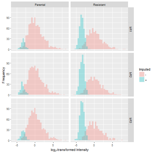
df.FNI = impute_data(df.FN)
Let's graphically evaluate the results by overlaying the distribution of the imputed values over the original distribution. In doing so, we observe that the number of missing values is greater in the resistant condition compared to the control. Furthermore, the missing values take on a narrow spread at the lower end of the sample distribution, which reflects our notion that low levels of protein expression produce missing data.
Summary
This is the second of three tutorials on proteomics data analysis. I have described the approach to handling the missing value problem in proteomics.
In the final tutorial, we are ready to compare protein expression between the drug-resistant and the control lines. This involves performing a two-sample Welch's t-test on our data to extract proteins that are differentially expressed. Moreover, we will discuss ways to interpret the final output of a high-throughput proteomics experiment. Stay tuned for the revelation of proteins that may play a role in driving the resistance of tumor cells.