The analysis of DNA and RNA, the blueprint of life and its carbon copy, has become a staple in the burgeoning field of molecular biology. An emerging and exciting area of study that adds another dimension to our understanding of cellular biology is that of proteomics, or the study of proteins inside the cell. The use of mass spectrometry has enabled the identification and quantification of thousands of proteins in a single experiment.
In this tutorial series, I will break down the steps to process a high-throughput proteomics data set derived from mass spectrometry analysis as follows:
- Data acquisition and cleaning
- Data filtering and missing value imputation
- Statistical testing and data interpretation
Source of Proteomics Data
To obtain a sample data set, I combed through a proteomics data repository called PRIDE and found an interesting study on drug resistance in breast cancer cell lines. I downloaded the raw files, which are the output of mass spectrometry analysis, and processed them using a software called MaxQuant to map the spectral data to protein sequences. A total of six raw files, corresponding to two conditions (one resistant line and one control) with three replicates each, were used. There are numerous other tools for processing mass spectrometry data (e.g. Mascot, SEQUEST, ProteinProspector), and the final data table of protein abundance measurements will vary base on the approach. The starting point for this tutorial is the MaxQuant ProteinGroups output file, which can be downloaded here.
Data Acquisition
The first step is to read the tab-separated data file into R.
# Read raw file
raw = read.delim("proteinGroups.txt", stringsAsFactors = FALSE, colClasses = "character")
Our raw data is an enormous 1787-by-79 data frame. Proteins are arranged in rows and the descriptors in columns. The primary columns of interest are those containing intensity measurements, which reflect protein abundances.
# Extract names of intensity columns
grep("^LFQ.intensity", names(raw), value = TRUE)
## [1] "LFQ.intensity.Parental_bR1"  "LFQ.intensity.Parental_bR2"
## [3] "LFQ.intensity.Parental_bR3"  "LFQ.intensity.Resistant_bR1"
## [5] "LFQ.intensity.Resistant_bR2" "LFQ.intensity.Resistant_bR3"
Again, we have a total of six samples. The Parental represents intensity data from the breast cancer cell line SKBR3 while the Resistant is an drug-resistant cell line derived from culturing the parentals in the presence of an inhibitor. This small molecule targets epidermal growth factor receptor (EGFR), a cell-surface protein that is frequently over-expressed in breast tumors leading to increased cell proliferation. For more information regarding the study, please see the original publication.
Data Cleaning
Remove False Hits
The next step after data acquisition is to clean and organize our data. The first order of business is to remove false hits, including contaminants, reverse proteins, and proteins identified by site. These are annotated with a “+” under the columns Potential.contaminant, Reverse, and Only.identified.by.site. We filter the data frame by keeping rows without a “+” annotation in any of the three columns.
library(dplyr)   # for data manipulation

# Filter false hits
df = raw %>%
  filter(Potential.contaminant != "+") %>%
  filter(Reverse != "+") %>%
  filter(Only.identified.by.site != "+")
Often there is a column that indicates the confidence in protein identification. In our case, Q.value represents the probability that the protein is a false hit. A typical cutoff is set at 0.01. Fortunately, MaxQuant takes care of this operation and ensures that all Q values are below the threshold.
# Summary of Q values
summary(as.numeric(df$Q.value))
##      Min.   1st Qu.    Median      Mean   3rd Qu.      Max.
## 0.0000000 0.0000000 0.0000000 0.0007193 0.0012759 0.0091429
Extract Protein and Gene IDs
A quick look at Protein.IDs and Fasta.headers columns tells us that the protein IDs, protein names, and gene IDs are all lumped together.
# View first 6 entries in Protein.IDs
head(df$Protein.IDs)
## [1] "sp|A0AV96|RBM47_HUMAN" "sp|A0FGR8|ESYT2_HUMAN" "sp|A1L0T0|ILVBL_HUMAN"
## [4] "sp|A4D1S0|KLRG2_HUMAN" "sp|A5YKK6|CNOT1_HUMAN" "sp|A6NDG6|PGP_HUMAN"
# View first 6 entries in Fasta.headers
head(df$Fasta.headers)
## [1] ">sp|A0AV96|RBM47_HUMAN RNA-binding protein 47 OS=Homo sapiens GN=RBM47 PE=1 SV=2"
## [2] ">sp|A0FGR8|ESYT2_HUMAN Extended synaptotagmin-2 OS=Homo sapiens GN=ESYT2 PE=1 SV=1"
## [3] ">sp|A1L0T0|ILVBL_HUMAN Acetolactate synthase-like protein OS=Homo sapiens GN=ILVBL PE=1 SV=2"
## [4] ">sp|A4D1S0|KLRG2_HUMAN Killer cell lectin-like receptor subfamily G member 2 OS=Homo sapiens GN=KLRG2 PE=1 SV=3"
## [5] ">sp|A5YKK6|CNOT1_HUMAN CCR4-NOT transcription complex subunit 1 OS=Homo sapiens GN=CNOT1 PE=1 SV=2"
## [6] ">sp|A6NDG6|PGP_HUMAN Glycerol-3-phosphate phosphatase OS=Homo sapiens GN=PGP PE=1 SV=1"
We will use regular expressions to extract the protein names into a column named Protein.name, the UniProt protein IDs into Protein, and the gene IDs into Gene. Note that some rows are associated with multiple identifiers separated by semicolons. In those instances, we will isolate the first entry.
# Isolate the first entry
df$Protein.IDs = sub(";.*", "", df$Protein.IDs)
df$Fasta.headers = sub(";.*", "", df$Fasta.headers)

# Extract Protein name
regex = regexpr("(?<=_HUMAN.).*(?=.OS)", df$Fasta.headers, perl = TRUE)
df$Protein.name = regmatches(df$Fasta.headers, regex)

# Extract UniProtID
regex = regexpr("(?<=\\|).*(?=\\|)", df$Protein.IDs, perl = TRUE)
df$Protein = regmatches(df$Protein.IDs, regex)

# Extract Gene ID
regex = regexpr("((?<=\\|[[:alnum:]]{6}\\|).*(?=_HUMAN)|(?<=\\|[[:alnum:]]{10}\\|).*(?=_HUMAN))",
                df$Protein.IDs, perl = TRUE)
df$Gene = regmatches(df$Protein.IDs, regex)
Transform Intensity Columns
Due to our function call for reading the data table, all columns are cast as the character data type. We will convert the intensity columns to the numeric data type for downstream analysis.
# Extract names of intensity columns
intensity.names = grep("^LFQ.intensity", names(df), value = TRUE)

# Cast as numeric
df[intensity.names] = sapply(df[intensity.names], as.numeric)
Now let’s examine the distribution of protein intensities in a sample. Below is a histogram of the protein intensities in the Parental_bR1 sample.
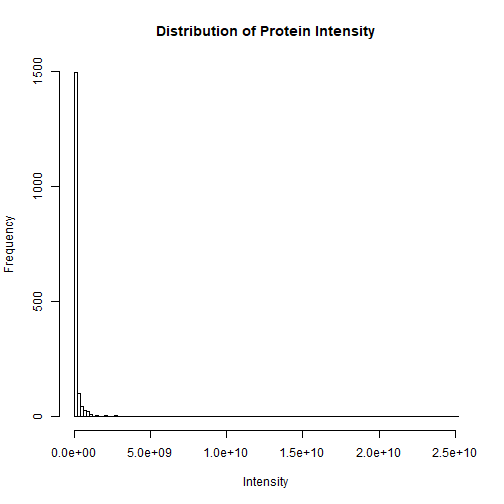
The distribution is clearly skewed to the right with a few highly abundant proteins. To normalize the distribution, it is common practice to log2-transform the intensity data.
# Assign column names for log2-transformed data
LOG.names = sub("^LFQ.intensity", "LOG2", intensity.names)   # rename intensity columns

# Transform data
df[LOG.names] = log2(df[intensity.names])
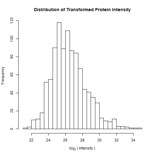
Here’s the transformed distribution on Parental_bR1 (much better!):
Summary
This is the first of three tutorials on proteomics data analysis. I have outlined the steps to read and clean a typical mass spectrometry-based proteomics data set.
In the next tutorial, we will examine the data in greater detail. In doing so, we will find that only a handful of proteins are quantified across all samples. In other words, proteins are often picked up in one sample but not in the others. This is known as the missing value problem. Stick around to learn the techniques for filtering proteins based on the number of valid values and filling in the missing values using data imputation.