A neural network is a computational system that creates predictions based on existing data. Let us train and test a neural network using the neuralnet library in R.
How To Construct A Neural Network?
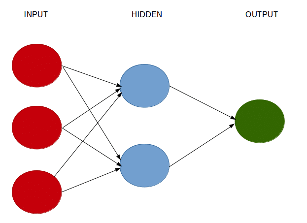
A neural network consists of:
- Input layers: Layers that take inputs based on existing data
- Hidden layers: Layers that use backpropagation to optimise the weights of the input variables in order to improve the predictive power of the model
- Output layers: Output of predictions based on the data from the input and hidden layers
Solving classification problems with neuralnet
In this particular example, our goal is to develop a neural network to determine if a stock pays a dividend or not.
As such, we are using the neural network to solve a classification problem. By classification, we mean ones where the data is classified by categories. e.g. a fruit can be classified as an apple, banana, orange, etc.
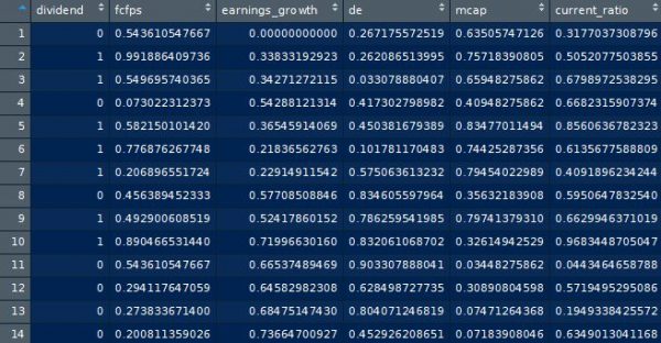
In our dataset, we assign a value of 1 to a stock that pays a dividend. We assign a value of 0 to a stock that does not pay a dividend. The dataset for this example is available at dividendinfo.csv.
Our independent variables are as follows:
- fcfps: Free cash flow per share (in $)
- earnings_growth: Earnings growth in the past year (in %)
- de: Debt to Equity ratio
- mcap: Market Capitalization of the stock
- current_ratio: Current Ratio (or Current Assets/Current Liabilities)
We firstly set our directory and load the data into the R environment:
setwd("your directory")
mydata <- read.csv("dividendinfo.csv")
attach(mydata)
Let’s now take a look at the steps we will follow in constructing this model.
Data Normalization
One of the most important procedures when forming a neural network is data normalization. This involves adjusting the data to a common scale so as to accurately compare predicted and actual values. Failure to normalize the data will typically result in the prediction value remaining the same across all observations, regardless of the input values.
We can do this in two ways in R:
- Scale the data frame automatically using the scale function in R
- Transform the data using a max-min normalization technique
We implement both techniques below but choose to use the max-min normalization technique. Please see this useful link for further details on how to use the normalization function.
Scaled Normalization
scaleddata<-scale(mydata)
Max-Min Normalization
For this method, we invoke the following function to normalize our data:
normalize <- function(x) {
  return ((x - min(x)) / (max(x) - min(x)))
}
Then, we use lapply to run the function across our existing data (we have termed the dataset loaded into R as mydata):
maxmindf <- as.data.frame(lapply(mydata, normalize))
We have now scaled our new dataset and saved it into a data frame titled maxmindf:
We base our training data (trainset) on 80% of the observations. The test data (testset) is based on the remaining 20% of observations.
# Training and Test Data
trainset <- maxmindf[1:160, ]
testset <- maxmindf[161:200, ]
Training a Neural Network Model using neuralnet
We now load the neuralnet library into R.
Observe that we are:
- Using neuralnet to “regress” the dependent “dividend” variable against the other independent variables
- Setting the number of hidden layers to (2,1) based on the hidden=(2,1) formula
- The linear.output variable is set to FALSE, given the impact of the independent variables on the dependent variable (dividend) is assumed to be non-linear
- The threshold is set to 0.01, meaning that if the change in error during an iteration is less than 1%, then no further optimization will be carried out by the model
Deciding on the number of hidden layers in a neural network is not an exact science. In fact, there are instances where accuracy will likely be higher without any hidden layers. Therefore, trial and error plays a significant role in this process.
One possibility is to compare how the accuracy of the predictions change as we modify the number of hidden layers.
For instance, using a (2,1) configuration ultimately yielded 92.5% classification accuracy for this example.
#Neural Network
library(neuralnet)
nn <- neuralnet(dividend ~ fcfps + earnings_growth + de + mcap + current_ratio, data=trainset, hidden=c(2,1), linear.output=FALSE, threshold=0.01)
nn$result.matrix
plot(nn)
Our neural network looks like this:
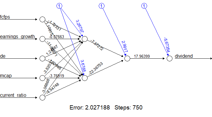
We now generate the error of the neural network model, along with the weights between the inputs, hidden layers, and outputs:
nn$result.matrix
                                           1
error                         2.027188266758
reached.threshold             0.009190064608
steps                       750.000000000000
Intercept.to.1layhid1         3.287965374794
fcfps.to.1layhid1            -1.723307330428
earnings_growth.to.1layhid1  -0.076629853467
de.to.1layhid1                1.243670462201
mcap.to.1layhid1             -3.520369700429
current_ratio.to.1layhid1    -3.068677865885
Intercept.to.1layhid2         3.618803162161
fcfps.to.1layhid2             1.109150492946
earnings_growth.to.1layhid2 -11.588713924832
de.to.1layhid2               -1.526458929898
mcap.to.1layhid2             -3.769192938001
current_ratio.to.1layhid2    -4.547481937028
Intercept.to.2layhid1         2.991704593713
1layhid.1.to.2layhid1        -7.372717428050
1layhid.2.to.2layhid1       -22.367528820159
Intercept.to.dividend        -5.673537382132
2layhid.1.to.dividend        17.963989719804
Testing The Accuracy Of The Model
As already mentioned, our neural network has been created using the training data. We then compare this to the test data to gauge the accuracy of the neural network forecast.
In the below:
- The “subset” function is used to eliminate the dependent variable from the test data
- The “compute” function then creates the prediction variable
- A “results” variable then compares the predicted data with the actual data
- A confusion matrix is then created with the table function to compare the number of true/false positives and negatives
#Test the resulting output
temp_test <- subset(testset, select = c("fcfps","earnings_growth", "de", "mcap", "current_ratio"))
head(temp_test)
nn.results <- compute(nn, temp_test)
results <- data.frame(actual = testset$dividend, prediction = nn.results$net.result)
The predicted results are compared to the actual results:
results
    actual     prediction
161      0 0.003457573932
162      1 0.999946522139
163      0 0.006824520245
...
198      0 0.005474975456
199      0 0.003427332586
200      1 0.999985252611
Confusion Matrix
Then, we round up our results using sapply and create a confusion matrix to compare the number of true/false positives and negatives:
roundedresults<-sapply(results,round,digits=0)
roundedresultsdf=data.frame(roundedresults)
attach(roundedresultsdf)
table(actual,prediction)
      prediction
actual  0  1
     0 17  0
     1  3 20
A confusion matrix is used to determine the number of true and false positives generated by our predictions. The model generates 17 true negatives (0’s), 20 true positives (1’s), while there are 3 false negatives.
Ultimately, we yield an 92.5% (37/40) accuracy rate in determining whether a stock pays a dividend or not.
Solving regression problems using neuralnet
We have already seen how a neural network can be used to solve classification problems by attempting to group data based on its attributes. However, what if we wish to solve a regression problem using a neural network? i.e. one where the dependent variable is an interval one and can take on a wide range of values?
Let us now visit the gasoline.csv dataset. In this example, we wish to analyze the impact of the explanatory variables capacity, gasoline, and hours on the dependent variable consumption.
Essentially, we wish to determine the gasoline spend per year (in $) for a particular vehicle based on different factors.
Accordingly, our variables are as follows:
- consumption: Spend (in $) on gasoline per year for a particular vehicle
- capacity: Capacity of the vehicle’s fuel tank (in litres)
- gasoline: Average cost of gasoline per pump
- hours: Hours driven per year by owner
Data Normalization
Again, we normalize our data and split into training and test data:
# MAX-MIN NORMALIZATION
normalize <- function(x) {
 return ((x - min(x)) / (max(x) - min(x)))
}
maxmindf <- as.data.frame(lapply(fullData, normalize))

# TRAINING AND TEST DATA
trainset <- maxmindf[1:32, ]
testset <- maxmindf[33:40, ]
Neural Network Output
We then run our neural network and generate our parameters:
#4. NEURAL NETWORK
library(neuralnet)
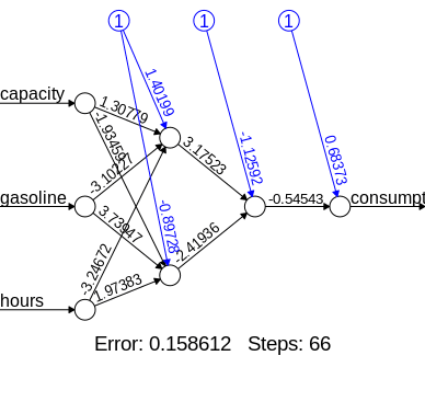
nn <- neuralnet(consumption ~ capacity + gasoline + hours,data=trainset, hidden=c(2,1), linear.output=TRUE, threshold=0.01)
nn$result.matrix
1
error 0.158611967443
reached.threshold 0.007331578682
steps 66.000000000000
Intercept.to.1layhid1 1.401987575173
capacity.to.1layhid1 1.307794013481
gasoline.to.1layhid1 -3.102267882386
hours.to.1layhid1 -3.246720660493
Intercept.to.1layhid2 -0.897276576566
capacity.to.1layhid2 -1.934594889387
gasoline.to.1layhid2 3.739470402932
hours.to.1layhid2 1.973830465259
Intercept.to.2layhid1 -1.125920206855
1layhid.1.to.2layhid1 3.175227041522
1layhid.2.to.2layhid1 -2.419360506652
Intercept.to.consumption 0.683726702522
2layhid.1.to.consumption -0.545431580477
Generated Neural Network
Here is what our neural network looks like in visual format:
Model Validation
Then, we validate (or test the accuracy of our model) by comparing the estimated gasoline spend yielded from the neural network to the actual spend as reported in the test output:
results <- data.frame(actual = testset$consumption, prediction = nn.results$net.result)
results
         actual   prediction
33 0.7556029883 0.6669224684
34 0.7801494130 0.6458686668
35 0.8356456777 0.6549105183
36 0.8399146211 0.6646982158
37 0.8431163287 0.6631168047
38 0.8890074707 0.6629885579
39 0.9124866596 0.6649999344
40 1.0000000000 0.6665075920
Accuracy
In the below code, we are then converting the data back to its original format, and yielding an accuracy of 90% on a mean absolute deviation basis (i.e. the average deviation between estimated and actual gasoline consumption stands at a mean of 10%). Note that we are also converting our data back into standard values given that they were previously scaled using the max-min normalization technique:
predicted=results$prediction * abs(diff(range(consumption))) + min(consumption)
actual=results$actual * abs(diff(range(consumption))) + min(consumption)
comparison=data.frame(predicted,actual)
deviation=((actual-predicted)/actual)
comparison=data.frame(predicted,actual,deviation)
accuracy=1-abs(mean(deviation))
accuracy
[1] 0.9017828022
You can see that we obtain 90% accuracy using a (2,1) hidden configuration. This is quite good, especially considering that our dependent variable is in the interval format. However, let’s see if we can get it higher!
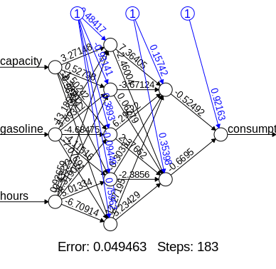
What happens if we now use a (5,2) hidden configuration in our neural network? Here is the generated output:
nn <- neuralnet(consumption ~ capacity + gasoline + hours,data=trainset, hidden=c(5,2), linear.output=TRUE, threshold=0.01)
nn$result.matrix
                                        1
error                      0.049463073770
reached.threshold          0.009079608691
steps                    183.000000000000
Intercept.to.1layhid1     -0.484165225327
capacity.to.1layhid1       3.271476705612
gasoline.to.1layhid1     -13.185417334090
hours.to.1layhid1          0.926588147188
Intercept.to.1layhid2     -0.931405056650
capacity.to.1layhid2       0.527977084370
gasoline.to.1layhid2       5.893120354012
hours.to.1layhid2         -0.435230849092
Intercept.to.1layhid3      0.389302962895
capacity.to.1layhid3      -1.502423111329
gasoline.to.1layhid3      -4.684748555999
hours.to.1layhid3         -6.319048800780
Intercept.to.1layhid4     -0.094490811578
capacity.to.1layhid4      -2.399916325456
gasoline.to.1layhid4      -4.115161295471
hours.to.1layhid4          5.013344559754
Intercept.to.1layhid5      0.759624731279
capacity.to.1layhid5      -0.565467044104
gasoline.to.1layhid5      -7.076912238164
hours.to.1layhid5         -6.709144936619
Intercept.to.2layhid1      0.157424617083
1layhid.1.to.2layhid1      7.364054381868
1layhid.2.to.2layhid1     -3.671237007644
1layhid.3.to.2layhid1      6.295218032535
1layhid.4.to.2layhid1     -0.303371875453
1layhid.5.to.2layhid1     12.271950628363
Intercept.to.2layhid2      0.353976458576
1layhid.1.to.2layhid2     -2.460042549015
1layhid.2.to.2layhid2      0.062791089253
1layhid.3.to.2layhid2      2.376623876363
1layhid.4.to.2layhid2     -2.385599836002
1layhid.5.to.2layhid2      5.234292659554
Intercept.to.consumption   0.921627990820
2layhid.1.to.consumption  -0.524918897571
2layhid.2.to.consumption  -0.669503028647
results <- data.frame(actual = testset$consumption, prediction = nn.results$net.result)
results
         actual   prediction
33 0.7556029883 0.6554040151
34 0.7801494130 0.7781191265
35 0.8356456777 0.7611519348
36 0.8399146211 0.7980981880
37 0.8431163287 0.8027250788
38 0.8890074707 0.8047567120
39 0.9124866596 0.7969363797
40 1.0000000000 0.7802800479
predicted=results$prediction * abs(diff(range(consumption))) + min(consumption)
actual=results$actual * abs(diff(range(consumption))) + min(consumption)
comparison=data.frame(predicted,actual)
deviation=((actual-predicted)/actual)
comparison=data.frame(predicted,actual,deviation)
accuracy=1-abs(mean(deviation))
accuracy
[1] 0.9577401232
We see that our accuracy rate has now increased to nearly 96%, indicating that modifying the number of hidden nodes has enhanced our model!
Conclusion
In this tutorial, you have learned how to use a neural network to solve classification problems.
Specifically, you saw how we can:
- Normalize data for meaningful analysis
- Classify data using a neural network
- Test accuracy using a confusion matrix
- Determine accuracy when the dependent variable is in interval format
Many thanks for viewing this tutorial.