It is often the case that a dataset contains significant outliers – or observations that are significantly out of range from the majority of other observations in our dataset. Let us see how we can use robust regressions to deal with this issue.
Plots
A useful way of dealing with outliers is by running a robust regression, or a regression that adjusts the weights assigned to each observation in order to reduce the skew resulting from the outliers.
In this particular example, we will build a regression to analyse internet usage in megabytes across different observations. You will see that we have several outliers in this dataset. Specifically, we have three incidences where internet consumption is vastly higher than other observations in the dataset.
Let’s see how we can use a robust regression to mitigate for these outliers.
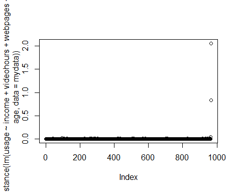
Firstly, let’s plot Cook’s distance and the QQ Plot:
Cook’s Distance
QQ Plot
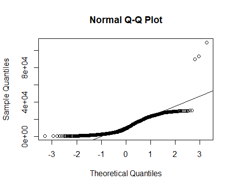
We can see that a plot of Cook’s distance shows clear outliers, and the QQ plot demonstrates the same (with a significant number of our observations not lying on the regression line).
When we get a summary of our data, we see that the maximum value for usage sharply exceeds the mean or median:
summary(mydata)
      age            gender          webpages
 Min.   :19.00   Min.   :0.0000   Min.   : 10.00
 1st Qu.:27.00   1st Qu.:0.0000   1st Qu.: 20.00
 Median :37.00   Median :1.0000   Median : 25.00
 Mean   :37.94   Mean   :0.5124   Mean   : 29.64
 3rd Qu.:48.75   3rd Qu.:1.0000   3rd Qu.: 32.00
 Max.   :60.00   Max.   :1.0000   Max.   :950.00
   videohours          income          usage
 Min.   : 0.0000   Min.   :    0   Min.   :   500
 1st Qu.: 0.4106   1st Qu.: 3503   1st Qu.:  3607
 Median : 1.7417   Median : 6362   Median :  9155
 Mean   : 4.0229   Mean   : 6179   Mean   : 11955
 3rd Qu.: 4.7765   3rd Qu.: 8652   3rd Qu.: 19361
 Max.   :45.0000   Max.   :12000   Max.   :108954
OLS Regression
Let’s now run a standard OLS regression and see what we come up with.
#OLS Regression
summary(ols <- lm(usage ~ income + videohours + webpages + gender + age, data = mydata))
Call:
lm(formula = usage ~ income + videohours + webpages + gender +
    age, data = mydata)

Residuals:
   Min     1Q Median     3Q    Max
-10925  -2559   -479   2266  46030

Coefficients:
              Estimate Std. Error t value Pr(>|t|)
(Intercept) -2.499e+03  4.893e+02  -5.107 3.96e-07 ***
income       7.874e-01  4.658e-02  16.903  < 2e-16 ***
videohours   1.172e+03  3.010e+01  38.939  < 2e-16 ***
webpages     5.414e+01  3.341e+00  16.208  < 2e-16 ***
gender      -1.227e+02  2.650e+02  -0.463    0.643
age          8.781e+01  1.116e+01   7.871 9.50e-15 ***
---
Signif. codes:  0 ‘***’ 0.001 ‘**’ 0.01 ‘*’ 0.05 ‘.’ 0.1 ‘ ’ 1

Residual standard error: 4113 on 960 degrees of freedom
Multiple R-squared:  0.8371,	Adjusted R-squared:  0.8363
F-statistic: 986.8 on 5 and 960 DF,  p-value: < 2.2e-16
We see that along with the estimates, most of our observations are significant at the 5% level and the R-Squared is reasonably high at 0.8371.
However, we need to bear in mind that this regression is not accounting for the fact that significant outliers exist in our dataset.
Cook’s Distance
A method we can use to determine outliers in our dataset is Cook’s distance. As a rule of thumb, if Cook’s distance is greater than 1, or if the distance in absolute terms is significantly greater than others in the dataset, then this is a good indication that we are dealing with an outlier.
#Compute Cooks Distance
dist <- cooks.distance(ols)
dist<-data.frame(dist)
]s <- stdres(ols)
a <- cbind(mydata, dist, s)

#Sort in order of standardized residuals
sabs <- abs(s)
a <- cbind(mydata, dist, s, sabs)
asorted <- a[order(-sabs), ]
asorted[1:10, ]
    age gender webpages videohours income  usage        dist
966  35      0       80 45.0000000   6700 108954 2.058817511
227  32      1       27  0.0000000   7830  24433 0.010733761
93   37      1       30  0.0000000  10744  27213 0.018822466
419  25      1       20  0.4952778   1767  17843 0.010178820
568  36      1       37  1.6666667   8360  25973 0.007652459
707  42      1       40  4.2347222   8527  29626 0.006085165
283  39      0       46  0.0000000   6244  22488 0.007099847
581  40      0       24  0.0000000   9746  23903 0.010620785
513  29      1       23  1.1111111  11398  25182 0.015107423
915  30      0       42  0.0000000   9455  22821 0.010412391
            s      sabs
966 11.687771 11.687771
227  4.048576  4.048576
93   4.026393  4.026393
419  3.707761  3.707761
568  3.627891  3.627891
707  3.583459  3.583459
283  3.448079  3.448079
581  3.393124  3.393124
513  3.353123  3.353123
915  3.162762  3.162762
We are adding Cook’s distance and standardized residuals to our dataset. Observe that we have the highest Cook’s distance and the highest standaridized residual for the observation with the greatest internet usage.
Huber and Bisquare Weights
At this point, we can now adjust the weights assigned to each observation to adjust our regression results accordingly.
Let’s see how we can do this using Huber and Bisquare weights.
Huber Weights
#Huber Weights
summary(rr.huber <- rlm(usage ~ income + videohours + webpages + gender + age, data = mydata))
Call: rlm(formula = usage ~ income + videohours + webpages + gender +
    age, data = mydata)
Residuals:
     Min       1Q   Median       3Q      Max
-11605.7  -2207.7   -177.2   2430.9  49960.3

Coefficients:
            Value      Std. Error t value
(Intercept) -3131.2512   423.0516    -7.4016
income          0.9059     0.0403    22.4945
videohours   1075.0703    26.0219    41.3140
webpages       57.1909     2.8880    19.8028
gender       -173.4154   229.0994    -0.7569
age            88.6238     9.6455     9.1881

Residual standard error: 3449 on 960 degrees of freedom
huber <- data.frame(usage = mydata$usage, resid = rr.huber$resid, weight = rr.huber$w)
huber2 <- huber[order(rr.huber$w), ]
huber2[1:10, ]
     usage    resid     weight
966 108954 49960.32 0.09284397
227  24433 16264.20 0.28518764
93   27213 15789.65 0.29375795
419  17843 15655.03 0.29628629
707  29626 14643.43 0.31675392
568  25973 14605.87 0.31756653
283  22488 13875.58 0.33427984
581  23903 13287.62 0.34907331
513  25182 13080.99 0.35458486
105  19606 12478.59 0.37170941
Bisquare weighting
#Bisquare weighting
rr.bisquare <- rlm(usage ~ income + videohours + webpages + gender + age, data=mydata, psi = psi.bisquare)
summary(rr.bisquare)
Call: rlm(formula = usage ~ income + videohours + webpages + gender +
    age, data = mydata, psi = psi.bisquare)
Residuals:
     Min       1Q   Median       3Q      Max
-11473.6  -2177.8   -119.7   2491.9  50000.1

Coefficients:
            Value      Std. Error t value
(Intercept) -3204.9051   426.9458    -7.5066
income          0.8985     0.0406    22.1074
videohours   1077.1598    26.2615    41.0167
webpages       56.3637     2.9146    19.3384
gender       -156.7096   231.2082    -0.6778
age            90.2113     9.7343     9.2673

Residual standard error: 3434 on 960 degrees of freedom
bisqr <- data.frame(usage = mydata$usage, resid = rr.bisquare$resid, weight = rr.bisquare$w)
bisqr2 <- bisqr[order(rr.bisquare$w), ]
bisqr2[1:10, ]
     usage    resid       weight
227  24433 16350.56 0.0000000000
966 108954 50000.09 0.0000000000
93   27213 15892.10 0.0005829225
419  17843 15700.87 0.0022639112
707  29626 14720.97 0.0264753021
568  25973 14694.59 0.0274546293
283  22488 13971.53 0.0604133298
581  23903 13389.67 0.0944155930
513  25182 13192.86 0.1072333000
105  19606 12536.39 0.1543038994
In both of the above instances, observe that a much lower weight of 0.092 is assigned to observation 966 using Huber weights, and a weight of 0 is assigned to the same observation using Bisquare weighting.
In this regard, we are allowing the respective regressions to adjust the weights in a way that yields lesser importance to outliers in our model.
Conclusion
In this tutorial, you have learned how to:
- Screen for outliers using Cook’s distance and QQ Plots
- Why standard linear regressions do not necessarily adjust for outliers
- How to use weighting techniques to adjust for such anomalies
If you have any questions on anything I have covered in this tutorial, please leave a comment and I will do my best to address your query.