One of the main limitations of regression analysis is when one needs to examine changes in data across several categories. This problem can be resolved by using a multilevel model, i.e. one that varies at more than one level and allows for variation between different groups or categories.
This dataset from data.ok.gov contains information on purchases made by state and higher educational institutions in the State of Oklahoma from various vendors.
Multilevel Model: Vendor Data
Consider the following business problem. Suppose that new vendors wish to enter the market and sell to these institutions. How can we estimate potential sales to these institutions by these new vendors? Let us see how using a multilevel model can help us accomplish this.
Firstly, the relevant libraries and dataset are imported.
# Import Libraries
library(lme4)
library(ggplot2)
library(reshape2)
library(dplyr)
library(data.table)

# Load data and convert to numeric
setwd("yourdirectory")
mydata<-read.csv("file.csv")
attach(mydata)
From this dataset, we are importing General Purchases across different agencies (as identified by their Agency Number), along with the Amount data (it is being assumed that all the positive values represent the purchases from these vendors).
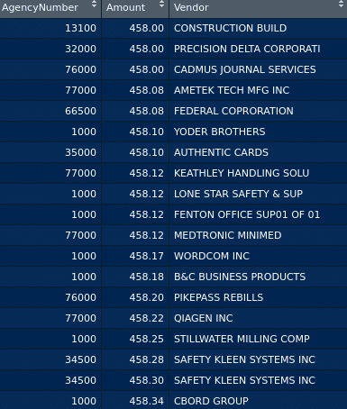
The Vendor variable is converted into numeric format and the data frame is formulated once again:
Vendor<-as.numeric(Vendor)
mydata<-data.frame(mydata,Vendor)
attach(mydata)
The multilevel model is formulated, and the conditional modes of the random effects are extracted using ranef.
mlevel <- lmer(Amount ~ 1 + (1|Vendor.1),mydata)
ranef(mlevel)
Here are the regression results:
mlevel
Linear mixed model fit by REML ['lmerMod']
Formula: Amount ~ 1 + (1 | Vendor.1)
   Data: mydata
REML criterion at convergence: 4967261
Random effects:
 Groups   Name        Std.Dev.
 Vendor.1 (Intercept) 4616
 Residual             5910
Number of obs: 244051, groups:  Vendor.1, 39789
Fixed Effects:
(Intercept)
      574.2
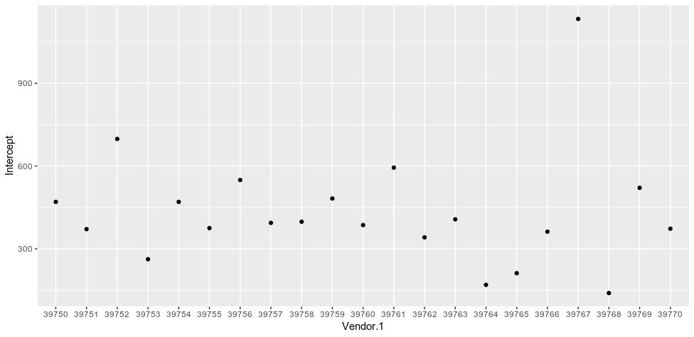
For the purchase data, the fixed and random effects are added together, and a plot of purchases for the last 20 observations are formulated.
# Average sales (amount) by vendor
purchases <- fixef(mlevel) + ranef(mlevel)$Vendor.1
purchases$Vendor.1<-rownames(purchases)
names(purchases)[1]<-"Intercept"
purchases <- purchases[,c(2,1)]
# plot
ggplot(purchases[39750:39770,],aes(x=Vendor.1,y=Intercept))+geom_point()
Now that the observed data has been generated, 20 simulations will be run to generate predictions for the 20 hypothetical new vendors – i.e. what sales could a new vendor to this market expect?
The fixed intercept is added to a random number with a standard deviation of 200:
# Simulation - 20 new vendors
new_purchases <- data.frame(Vendor.1 = as.character(39800:39819),
                          Intercept= fixef(mlevel)+rnorm(20,0,200),Status="Simulated")
purchases$Status <- "Observed"
purchases2 <- rbind(purchases,new_purchases)
Now, the simulated amounts can be plotted against observed amounts to determine potential vendor sales:
# Plot simulated vs observed
ggplot(purchases2[39709:39809,],aes(x=Vendor.1,y=Intercept,color=Status))+
  geom_point()+
  geom_hline(aes(yintercept = fixef(mlevel)[1],linewidth=1.5))
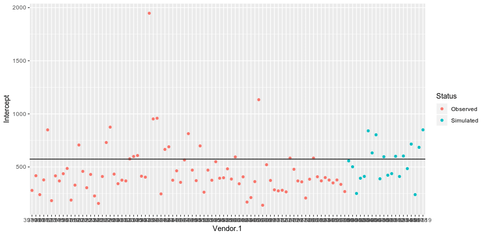
We can see that the simulated sales are more or less in line with that observed from the actual data. As mentioned, the advantage of a multilevel model is the fact that differences across levels are taken into account when running the model, and this helps us avoid the issue of significantly different trends across levels ultimately yielding a “one size fits all” result from a standard linear regression.
Conclusion
In this example, we have seen:
- How to implement a multilevel model in R
- The advantages of these models in modelling data with multiple categories
- Running simulations with the model
You can also find another example of how to run a multilevel model here.