In this post, I am going to run an exploratory analysis of the plant leaf dataset as made available by UCI Machine Learning repository at this link. The dataset is expected to comprise sixteen samples each of one-hundred plant species. Its analysis was introduced within ref. [1]. That paper describes a method designed to work in conditions of small training set size and possibly incomplete extraction of features.
This motivated separate processing of three feature types:
- shape
- texture
- margin
Those are then combined to provide an overall indication of the species (and associated probability). For an accurate description of those features, please see ref. [1] where the classification is implemented by a K-Nearest-Neighbor density estimator. Ref. [1] authors show the accuracy reached by K-Nearest-Neighbor classification for any combination of the datasets in use (see ref. [1] Table 2).
Packages
suppressPackageStartupMessages(library(caret))
suppressPackageStartupMessages(library(dplyr))
suppressPackageStartupMessages(library(ggplot2))
suppressPackageStartupMessages(library(corrplot))
suppressPackageStartupMessages(library(Hmisc))
Exploratory Analysis
Getting Data
We can download the leaf dataset as a zip file by taking advantage of the following UCI Machine Learning url.
url <- "https://archive.ics.uci.edu/ml/machine-learning-databases/00241/100%20leaves%20plant%20species.zip"
temp_file <- tempfile()
download.file(url, temp_file)
The files of interest are:
margin_file <- "100 leaves plant species/data_Mar_64.txt"
shape_file <- "100 leaves plant species/data_Sha_64.txt"
texture_file <- "100 leaves plant species/data_Tex_64.txt"
that can be so extracted.
files_to_unzip <- c(margin_file, shape_file, texture_file)
unzip(temp_file, files = files_to_unzip, exdir=".", overwrite = TRUE)
We read them as CSV files. No header is originally provided.
margin_data <- read.csv(margin_file, header=FALSE, sep=",", stringsAsFactors = TRUE)
shape_data <- read.csv(shape_file, header=FALSE, sep=",", stringsAsFactors = TRUE)
texture_data <- read.csv(texture_file, header=FALSE, sep=",", stringsAsFactors = TRUE)
We check the number of rows and columns of the resulting datasets.
dim(margin_data)
## [1] 1600   65
dim(shape_data)
## [1] 1600   65
dim(texture_data)
## [1] 1599   65
We notice that the texture dataset has one row less. Such issue will be fixed at a later moment.
sum(complete.cases(margin_data)) == nrow(margin_data)
## [1] TRUE
sum(complete.cases(shape_data)) == nrow(shape_data)
## [1] TRUE
sum(complete.cases(texture_data)) == nrow(texture_data)
## [1] TRUE
No NA's value are present. Column naming is necessary due to the absence of header.
n_features <- ncol(margin_data) - 1
colnames(margin_data) <- c("species", paste("margin", as.character(1:n_features), sep=""))
margin_data$species <- factor(margin_data$species)

n_features <- ncol(shape_data) - 1
colnames(shape_data) <- c("species", paste("shape", as.character(1:n_features), sep=""))
shape_data$species <- factor(shape_data$species)

n_features <- ncol(texture_data) - 1
colnames(texture_data) <- c("species", paste("texture", as.character(1:n_features), sep=""))
texture_data$species <- factor(texture_data$species)
We count the number of entries for each species within each dataset.
margin_count <- sapply(base::split(margin_data, margin_data$species), nrow)
shape_count <- sapply(base::split(shape_data, shape_data$species), nrow)
texture_count <- sapply(base::split(texture_data, texture_data$species), nrow)
That in order to identify what species is associated to the missing entry inside the texture dataset.
which(margin_count != texture_count)
## Acer Campestre
##              1
which(shape_count != texture_count)
## Acer Campestre
##              1
The texture data missing entry is associated to Acer Campestre species. Adding an identifier column to all datasets to allow for datasets merging (joining).
margin_data <- mutate(margin_data, id = 1:nrow(margin_data))
shape_data <- mutate(shape_data, id = 1:nrow(shape_data))
texture_data <- mutate(texture_data, id = 1:nrow(texture_data))
Imputation
In the following, we fix the missing entry by imputation technique based on median. We suppose the missing entry is related with 16th sample of Acer Campestre texture data, which is the first plant species of our datasets. For the purpose, we take advantage of a temporary dataset made of first 15 entries and then we add such new row with median computed data. Afterwards, we “row-bind” such temporary dataset with the rest of the original texture samples.
dd <- data.frame(matrix(nrow=1, ncol = 66))
colnames(dd) <- colnames(texture_data)
dd$species <- "Acer Campestre"
dd$id <- 16

temp_texture_data <- rbind(texture_data[1:15,], dd)
features <- setdiff(colnames(temp_texture_data), c("species", "id"))
imputed <- sapply(features, function(x) { as.numeric(impute(temp_texture_data[, x], median)[16])})
temp_texture_data[16, names(imputed)] <- imputed

texture_data <- rbind(temp_texture_data, texture_data[-(1:15),])
texture_data <- mutate(texture_data, id = 1:nrow(texture_data))
dim(texture_data)
## [1] 1600   66
Here is what we got at the end.
str(margin_data)
## 'data.frame':    1600 obs. of  66 variables:
##  $ species : Factor w/ 100 levels "Acer Campestre",..: 1 1 1 1 1 1 1 1 1 1 ...
##  $ margin1 : num  0.00391 0.00586 0.01172 0.01367 0.00781 ...
##  $ margin2 : num  0.00391 0.01367 0.00195 0.01172 0.00977 ...
##  $ margin3 : num  0.0273 0.0273 0.0273 0.0371 0.0273 ...
##  $ margin4 : num  0.0332 0.0254 0.0449 0.0176 0.0254 ...
##  $ margin5 : num  0.00781 0.01367 0.01758 0.01172 0.00195 ...
##  $ margin6 : num  0.01758 0.0293 0.04297 0.08789 0.00586 ...
##  $ margin7 : num  0.0234 0.0195 0.0234 0.0234 0.0156 ...
##  $ margin8 : num  0.00586 0 0 0 0 ...
##  $ margin9 : num  0 0.00195 0.00391 0 0.00586 ...
##  $ margin10: num  0.0156 0.0215 0.0195 0.0273 0.0176 ...
....
....
str(shape_data)
## 'data.frame':    1600 obs. of  66 variables:
##  $ species: Factor w/ 100 levels "Acer Campestre",..: 2 2 2 2 2 2 2 2 2 2 ...
##  $ shape1 : num  0.000579 0.00063 0.000616 0.000613 0.000599 ...
##  $ shape2 : num  0.000609 0.000661 0.000615 0.000569 0.000552 ...
##  $ shape3 : num  0.000551 0.000719 0.000606 0.000564 0.000558 ...
##  $ shape4 : num  0.000554 0.000651 0.000568 0.000607 0.000569 ...
##  $ shape5 : num  0.000603 0.000643 0.000558 0.000643 0.000616 ...
##  $ shape6 : num  0.000614 0.00064 0.000552 0.000647 0.000639 ...
##  $ shape7 : num  0.000611 0.000646 0.000551 0.000663 0.000631 ...
##  $ shape8 : num  0.000611 0.000624 0.000552 0.000658 0.000634 ...
##  $ shape9 : num  0.000611 0.000584 0.000531 0.000635 0.000639 ...
##  $ shape10: num  0.000594 0.000546 0.00053 0.0006 0.000596 ...
...
...
str(texture_data)
## 'data.frame':    1600 obs. of  66 variables:
##  $ species  : Factor w/ 100 levels "Acer Campestre",..: 1 1 1 1 1 1 1 1 1 1 ...
##  $ texture1 : num  0.02539 0.00488 0.01855 0.03516 0.03809 ...
##  $ texture2 : num  0.0127 0.0186 0.0137 0.0234 0.0146 ...
##  $ texture3 : num  0.003906 0.00293 0.00293 0.000977 0.003906 ...
##  $ texture4 : num  0.004883 0 0.00293 0 0.000977 ...
##  $ texture5 : num  0.0391 0.0693 0.0518 0.0615 0.0469 ...
##  $ texture6 : num  0 0 0 0 0 0 0 0 0 0 ...
##  $ texture7 : num  0.0176 0.0137 0.0195 0.0215 0.0225 ...
##  $ texture8 : num  0.0352 0.0439 0.0352 0.0615 0.0537 ...
##  $ texture9 : num  0.0234 0.0264 0.0225 0.0107 0.0195 ...
##  $ texture10: num  0.013672 0 0.000977 0.001953 0.004883 ...
...
...
Correlation Analysis
Since margin, shape and texture covariates are quantitative variables, it is of interest to evaluate correlation among such leaf features.
We do it by taking advantage of the correlation plot. We show that for the margin1 feature.
m_l <- split(margin_data, margin_data$species)

extract_feature <- function(m_l, feature) {
  f <- lapply(m_l, function(x) { x[,feature] })
  do.call(cbind, f)
}

thefeature <- "margin1"
m <- extract_feature(m_l, thefeature)
cor_mat <- cor(m)
corrplot(cor_mat, method = "circle", type="upper", tl.cex=0.3)
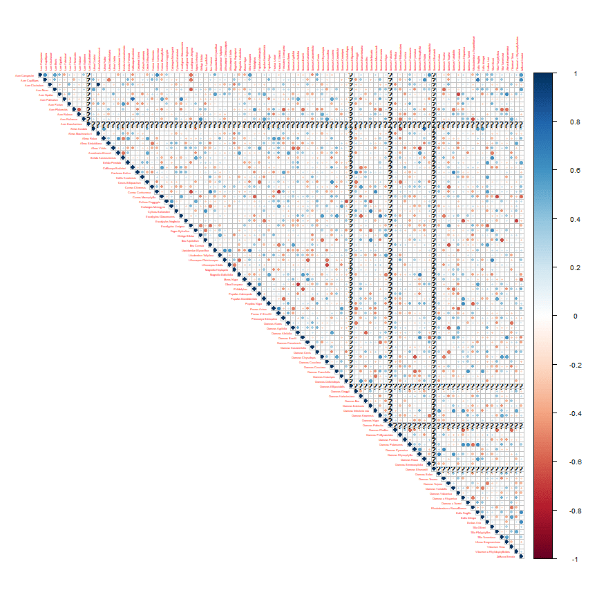
The correlation plot is not so easy to interpret. Therefore we implement a procedure capable to filter out the significative and most relevant correlations. At the purpose, we use an helper function named as flattenCorrMatrix as can be found in ref. [3].
flattenCorrMatrix <- function(cormat, pmat) {
  ut <- upper.tri(cormat)
  data.frame(
    row = rownames(cormat)[row(cormat)[ut]],
    column = rownames(cormat)[col(cormat)[ut]],
    cor  =(cormat)[ut],
    p = pmat[ut]
    )
}
The following utility function is capable to extract a given feature from one of the available datasets and report the flatten correlation matrix providing with the significative correlation and whose relevance is above a certain absolute value as specified by the threshold parameter.
most_correlated <- function(dataset, feature, threshold) {
  m_l <- split(dataset, dataset$species)
  m <- extract_feature(m_l, feature)
  rcorr_m <- rcorr(m)
  flat_cor <- flattenCorrMatrix(rcorr_m$r, rcorr_m$P)
  attr(flat_cor, "variable") <- feature
  flat_cor <- flat_cor %>% filter(p < 0.05) %>% filter(abs(cor) > threshold)
  flat_cor[,-4] # getting rid of the p-value column
}
Here is what we get as correlation matrix for the margin_data dataset and the margin2 feature with a threshold equal to 0.7.
corr_margin2 <- most_correlated(margin_data, "margin2", 0.7)
corr_margin2
##                    row                  column        cor
## 1      Acer Capillipes     Cercis Siliquastrum  0.7038700
## 2  Cercis Siliquastrum      Cornus Controversa -0.7294585
## 3            Acer Mono Liriodendron Tulipifera -0.7032354
## 4      Ilex Aquifolium             Morus Nigra  0.7647532
## 5          Acer Opalus   Populus Grandidentata -0.7751047
## 6  Cercis Siliquastrum            Prunus Avium  0.7295616
## 7     Cornus Chinensis   Pterocarya Stenoptera  0.7345398
## 8        Alnus Cordata         Quercus Brantii  0.7257876
## 9       Acer Campestre  Quercus Phillyraeoides -0.7150759
## 10     Acer Circinatum           Quercus Rubra  0.8082904
## 11  Cornus Controversa  Quercus Semecarpifolia -0.7089530
## 12     Castanea Sativa      Quercus Variabilis  0.7299116
## 13      Acer Rufinerve       Quercus Vulcanica  0.7180856
If we want to collect all the correlation matrixes for the margin_data, here is how we can do.
margin_names <- setdiff(colnames(margin_data), c("species", "id"))
margin_corr_l <- lapply(margin_names, function(x) {most_correlated(margin_data, x, 0.7)})
names(margin_corr_l) <- margin_names
Let us have a look at a correlation matrix as item of such list.
margin_corr_l[["margin32"]]
##                      row                       column        cor
## 1    Eucalyptus Urnigera                  Morus Nigra  0.7623514
## 2    Eucalyptus Urnigera                Olea Europaea  1.0000000
## 3            Morus Nigra                Olea Europaea  0.7623514
## 4    Cercis Siliquastrum            Quercus Agrifolia  0.7474093
## 5     Cornus Macrophylla              Quercus Brantii  0.8071712
## 6      Populus Adenopoda        Quercus Castaneifolia  0.7092994
## 7      Quercus Coccifera            Quercus Crassipes  0.7422717
## 8    Arundinaria Simonii        Quercus Ellipsoidalis  0.7625542
## 9     Cornus Controversa              Quercus Greggii  1.0000000
## 10             Acer Mono              Quercus Phellos  0.9165285
## 11     Quercus Crassipes       Quercus Semecarpifolia  0.7682705
## 12   Cytisus Battandieri            Quercus Shumardii -0.7324311
## 13          Quercus Ilex                Quercus Suber  0.8382549
## 14  Quercus Dolicholepis               Quercus Texana  0.7090909
## 15     Quercus Pubescens               Salix Intergra  0.7603719
## 16       Ilex Aquifolium           Tilia Platyphyllos  0.7939940
## 17    Cornus Macrophylla               Viburnum Tinus  0.8451543
## 18        Betula Pendula Viburnum x Rhytidophylloides -0.7224267
## 19 Populus Grandidentata              Zelkova Serrata  0.7453458
Here we do the same for shape and texture features datasets. For shape dataset we show shape3 feature correlation matrix result.
shape_names <- setdiff(colnames(shape_data), c("species", "id"))
shape_corr_l <- lapply(shape_names, function(x) {most_correlated(shape_data, x, 0.7)})
names(shape_corr_l) <- shape_names
shape_corr_l[["shape3"]]
##                       row                 column        cor
## 1          Acer Campestre    Arundinaria Simonii  0.7643580
## 2           Alnus Viridis   Callicarpa Bodinieri -0.7467261
## 3         Acer Platanoids            Morus Nigra -0.7674200
## 4    Magnolia Salicifolia           Prunus Avium  0.7306309
## 5            Prunus Avium  Pterocarya Stenoptera  0.7042563
## 6             Morus Nigra         Quercus Cerris -0.7316674
## 7       Quercus Alnifolia    Quercus Chrysolepis  0.7019743
## 8  Eucalyptus Glaucescens    Quercus Crassifolia  0.7414744
## 9          Quercus Cerris        Quercus Greggii  0.7100278
## 10         Quercus Cerris           Quercus Ilex -0.8346480
## 11  Quercus Castaneifolia Quercus Phillyraeoides  0.7305218
## 12     Cornus Macrophylla          Quercus Rubra  0.8231097
## 13            Morus Nigra         Quercus Texana  0.7232813
## 14          Populus Nigra        Quercus Trojana -0.7157611
## 15      Quercus Alnifolia      Quercus Vulcanica -0.7350224
## 16    Quercus Chrysolepis      Quercus Vulcanica -0.8157281
## 17  Quercus Castaneifolia     Ulmus Bergmanniana  0.7747396
For texture dataset we show texture19 feature correlation matrix result.
texture_names <- setdiff(colnames(texture_data), c("species", "id"))
texture_corr_l <- lapply(texture_names, function(x) {most_correlated(texture_data, x, 0.7)})
names(texture_corr_l) <- texture_names
texture_corr_l[["texture19"]]
##                          row                       column        cor
## 1              Acer Palmatum         Callicarpa Bodinieri -0.8069241
## 2         Cornus Macrophylla              Ilex Aquifolium  0.7243966
## 3     Eucalyptus Glaucescens      Liriodendron Tulipifera  0.7609341
## 4        Eucalyptus Urnigera    Lithocarpus Cleistocarpus  0.8353815
## 5                  Acer Mono                Olea Europaea  0.8007114
## 6                Alnus Rubra                Olea Europaea  0.7121676
## 7    Liquidambar Styraciflua          Quercus Chrysolepis  0.7252803
## 8         Magnolia Heptapeta             Quercus Coccinea  0.7512588
## 9         Magnolia Heptapeta          Quercus Crassifolia  0.8270324
## 10          Quercus Coccinea          Quercus Crassifolia  0.7479191
## 11 Lithocarpus Cleistocarpus            Quercus Crassipes  0.7031255
## 12         Cotinus Coggygria            Quercus Palustris  0.7104135
## 13         Alnus Sieboldiana            Quercus Pyrenaica  0.7401955
## 14              Ilex Cornuta              Quercus Trojana  0.7432011
## 15               Morus Nigra              Quercus Trojana  0.7238492
## 16           Quercus Greggii          Quercus x Hispanica  0.7396316
## 17         Quercus Pyrenaica                  Sorbus Aria  0.7345942
## 18       Eucalyptus Neglecta                Tilia Oliveri  0.7565882
## 19              Prunus Avium Viburnum x Rhytidophylloides -0.7451209
## 20             Alnus Viridis              Zelkova Serrata -0.7052669
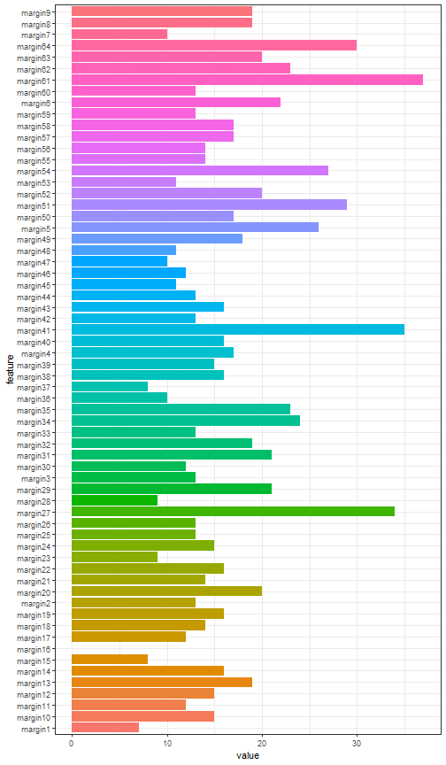
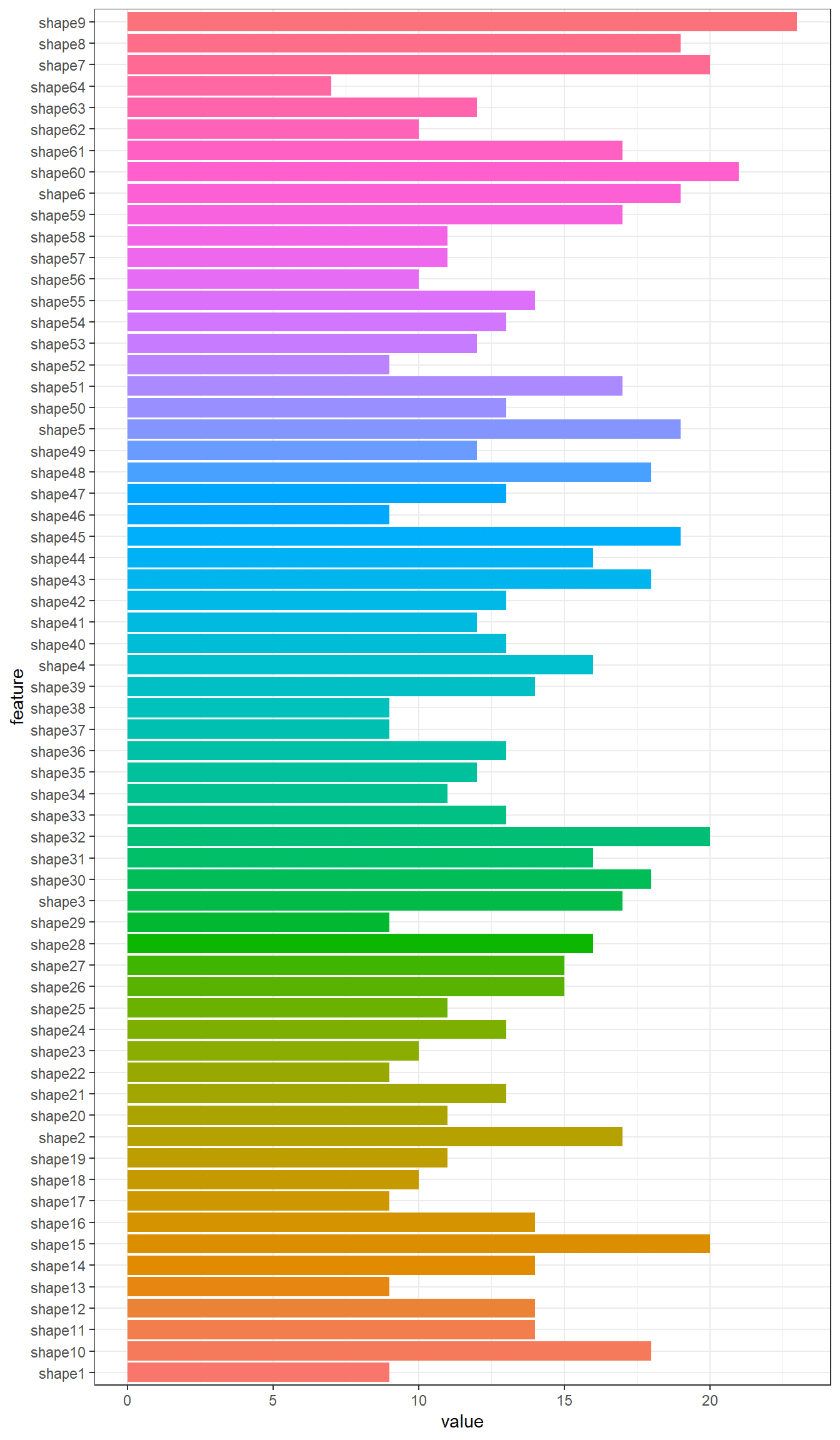
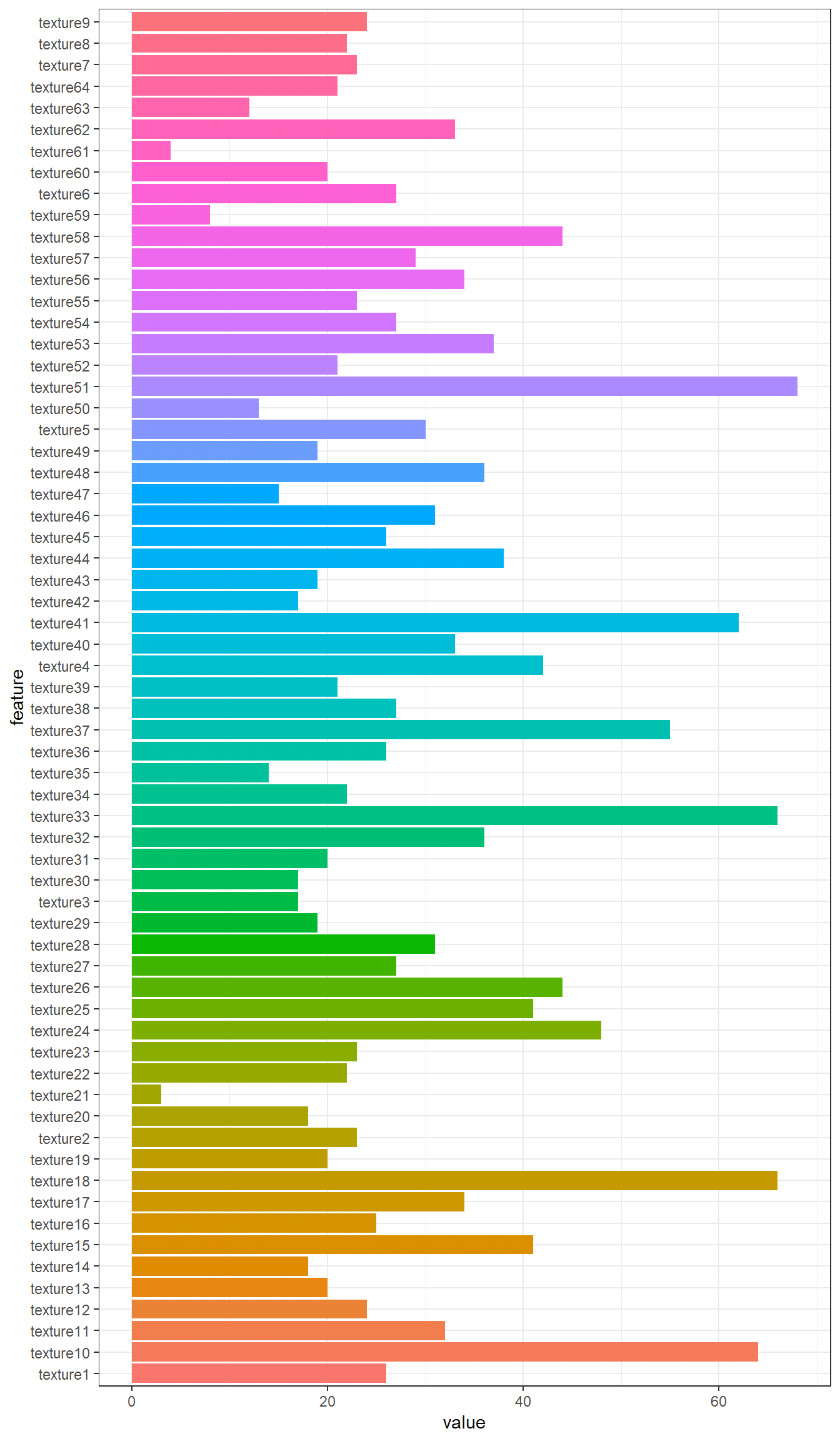
Furthermore, by collecting the number of rows of such correlation matrixes, the most correlated features among the one hundred leaf plant species can be put in evidence.
t <- sapply(margin_corr_l, nrow)
margin_c <- data.frame(feature = names(t), value = t)

t <- sapply(shape_corr_l, nrow)
shape_c <- data.frame(feature = names(t), value = t)

t <- sapply(texture_corr_l, nrow)
texture_c <- data.frame(feature = names(t), value = t)
ggplot(data = margin_c, aes(x=feature, y=value, fill = feature)) + theme_bw() + theme(legend.position = "none") + geom_histogram(stat='identity') + coord_flip()
ggplot(data = shape_c, aes(x=feature, y=value, fill = feature)) + theme_bw() + theme(legend.position = "none") + geom_histogram(stat='identity') + coord_flip()
ggplot(data = texture_c, aes(x=feature, y=value, fill = feature)) + theme_bw() + theme(legend.position = "none") + geom_histogram(stat='identity') + coord_flip()
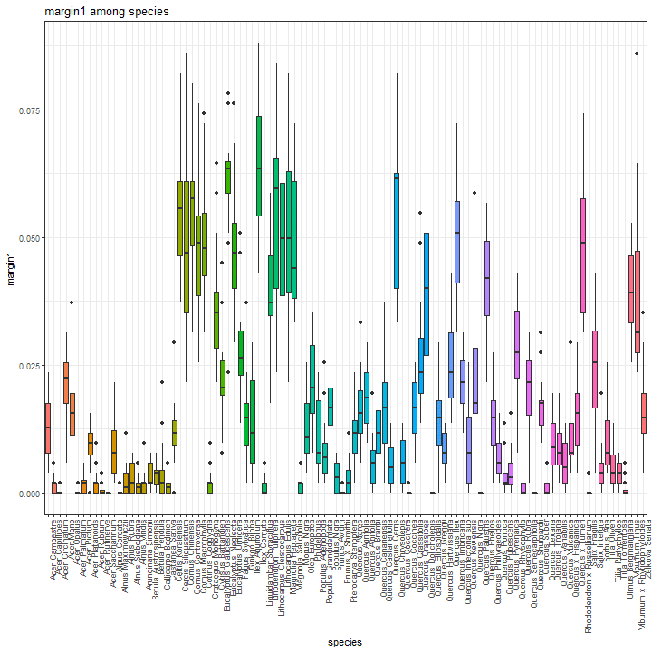
Boxplots are shown to highlight differences in features among species. At the purpose, we define the following utility function.
species_boxplot <- function(dataset, variable) {
  p <- ggplot(data = dataset, aes(x = species, y = eval(parse(text=variable)), fill= species)) + theme_bw() + theme(legend.position = "none") + geom_boxplot() + ylab(parse(text=variable))
  p <- p + theme(axis.text.x = element_text(angle = 90, hjust = 1)) + ggtitle(paste(variable, "among species", sep = " "))
  p
}
Margin feature boxplot
For each margin feature, a boxplot as shown below can be generated. Herein, the boxplot associated to the margin1 feature.
species_boxplot(margin_data, "margin1")
If you are interested in having a summary report, you may take advantage of the following line of code.
with(margin_data, tapply(margin1, species, summary))
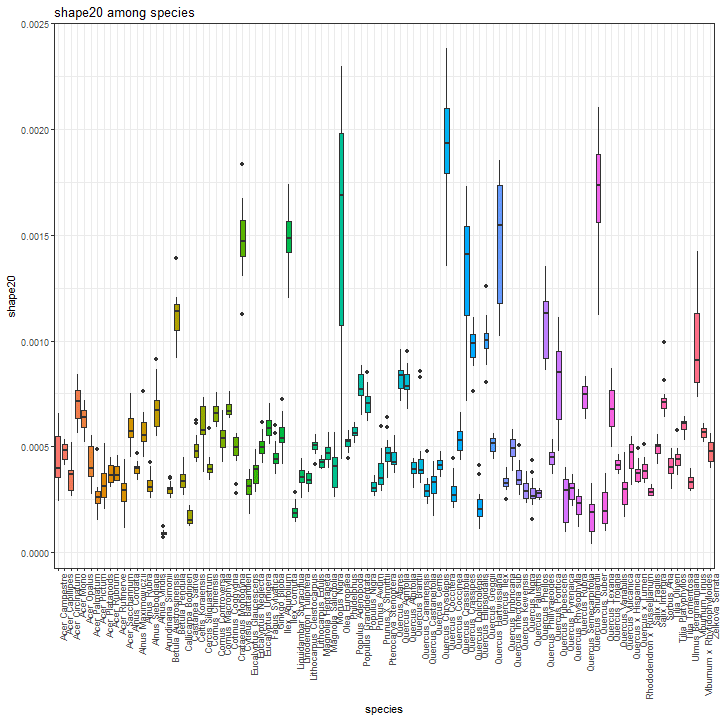
Shape feature boxplot
We show the boxplot for shape features by considering the shape20 as example.
species_boxplot(shape_data, "shape20")
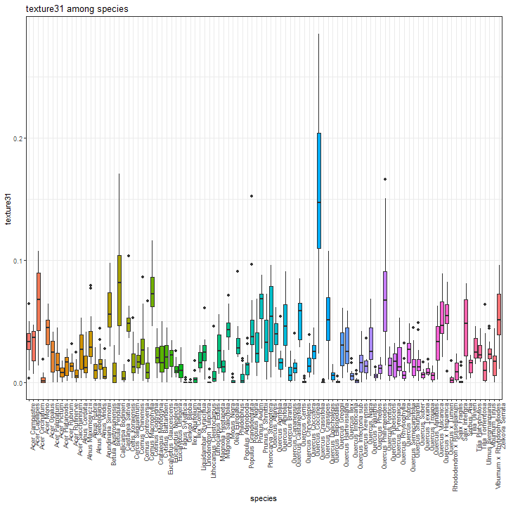
Texture feature boxplot
We show the boxplot for texture features by considering the texture31 as example.
species_boxplot(texture_data, "texture31")
Saving the current enviroment for further analysis.
save.image(file='PlantLeafEnvironment.RData')
References
- Charles Mallah, James Cope and James Orwell, “PLANT LEAF CLASSIFICATION USING PROBABILISTIC INTEGRATION OF SHAPE, TEXTURE AND MARGIN FEATURES”, link
- 100 Plant Leaf Dataset
- Correlation Matrix: a quick start guide