Data Science / Analytics is all about finding valuable insights from the given dataset. In short, Finding answers that could help business. In this tutorial, We will see how to get started with Data Analysis in Python. The Python packages that we use in this notebook are: numpy, pandas, matplotlib, and seaborn
Since usually such tutorials are based on in-built datasets like iris, It becomes harder for the learner to connect with the analysis and hence learning becomes difficult. To overcome this, The dataset that we use in this notebook is IPL (Indian Premier League) Dataset posted on Kaggle Datasets sourced from cricsheet. IPL is one of the most popular cricket tournaments in the world, thus the problems we try to solve and the questions that we try to answer should be familiar to anyone who knows Cricket.
Questions:
- How many matches we’ve got in the dataset?
- How many seasons we’ve got in the dataset?
- Which Team had won by maximum runs?
- Which Team had won by maximum wicket?
- Which Team had won by closest Margin (minimum runs)?
- Which Team had won by minimum wicket?
- Which Season had most number of matches?
- Which IPL Team is more successful?
- Has Toss-winning helped in winning matches?
Loading Libraries
Let us begin our analysis by loading the above mentioned Python Modules/Packages/Libraries.
import numpy as np # numerical computing
import pandas as pd # data processing, CSV file I/O (e.g. pd.read_csv)
import matplotlib.pyplot as plt #visualization
import seaborn as sns #modern visualization
To make our plots look nice, let us set a theme for our seaborn (sns) plots and also let us define the size in which we would like to print the plot figures.
sns.set_style("darkgrid")
plt.rcParams['figure.figsize'] = (14, 8)
Reading input dataset
In order to read the input data, let us first define the directory/path in which the input file is present. This is to make sure that the path is stored in a string first before using the same (concatenated) with the file name to read the input csv using pd.read_csv() function.
file_path = 'C:\\Users\\something\\Downloads\\'
matches = pd.read_csv(file_path+'matches.csv')
Get basic information of Data
To begin humbly, Let us check the basic information of the dataset. The very basic information to know is the dimension of the dataset – rows and columns – that’s what we find out with the method shape.
matches.shape
(636, 18)
And then, It’s important to know the different types of data/variables in the given dataset.
matches.info()
RangeIndex: 636 entries, 0 to 635
Data columns (total 18 columns):
id                 636 non-null int64
season             636 non-null int64
city               629 non-null object
date               636 non-null object
team1              636 non-null object
team2              636 non-null object
toss_winner        636 non-null object
toss_decision      636 non-null object
result             636 non-null object
dl_applied         636 non-null int64
winner             633 non-null object
win_by_runs        636 non-null int64
win_by_wickets     636 non-null int64
player_of_match    633 non-null object
venue              636 non-null object
umpire1            635 non-null object
umpire2            635 non-null object
umpire3            0 non-null float64
dtypes: float64(1), int64(5), object(12)
memory usage: 89.5+ KB
Moving one level up, let’s perform a simple summary statistics using the method describe().
matches.describe()
id
season
dl_applied
win_by_runs
win_by_wickets
umpire3
count
636.000000 636.000000 636.000000 636.000000 636.000000 0.0
mean
318.500000 2012.490566 0.025157 13.682390 3.372642 NaN
std
183.741666 2.773026 0.156726 23.908877 3.420338 NaN
min
1.000000 2008.000000 0.000000 0.000000 0.000000 NaN
25%
159.750000 2010.000000 0.000000 0.000000 0.000000 NaN
50%
318.500000 2012.000000 0.000000 0.000000 4.000000 NaN
75%
477.250000 2015.000000 0.000000 20.000000 7.000000 NaN
max
636.000000 2017.000000 1.000000 146.000000 10.000000 NaN
And the final level of this basic information retrieval is to see a couple of actual rows of the input dataset.
matches.head(2)
id
season
city
date
team1
team2
toss_winner
toss_decision
result
dl_applied
winner
win_by_runs
win_by_wickets
player_of_match
venue
umpire1
umpire2
umpire3
0
1 2017 Hyderabad 2017-04-05 Sunrisers Hyderabad Royal Challengers Bangalore Royal Challengers Bangalore field normal 0 Sunrisers Hyderabad 35 0 Yuvraj Singh Rajiv Gandhi International Stadium, Uppal AY Dandekar NJ Llong NaN
1
2 2017 Pune 2017-04-06 Mumbai Indians Rising Pune Supergiant Rising Pune Supergiant field normal 0 Rising Pune Supergiant 0 7 SPD Smith Maharashtra Cricket Association Stadium A Nand Kishore S Ravi NaN
Now, with the basic understanding of the input dataset. We are promoted to answer our questions with basic data analysis.
How many matches we’ve got in the dataset?
As we’ve seen above, id is a variable that counts each observation in the data while each observation is a match. So to get the number of matches in our dataset is as same as to get the number of rows in the dataset or maximum value of the variable id.
matches['id'].max()
636
636 IPL Matches is what we’ve got in our dataset.
How many seasons we’ve got in the dataset?
IPL like any other Sports league, happens once in a year and so getting the number of unique years we’ve got in the dataset will tell us how many seasons we’ve got in the dataset.
matches['season'].unique()
array([2017, 2008, 2009, 2010, 2011, 2012, 2013, 2014, 2015, 2016],
      dtype=int64)
That gives the list of years, but to answer the question with just the required answer, let’s calculate length of the list that was returned in the above step.
len(matches['season'].unique())
10
Which Team had won by maximum runs?
To answer this question, we can divide the question logically – first we need to find maximum runs, then we can find the row (winning team) with this maximum runs – which would indeed be the team won by maximum runs. I’d like to emphasis here that it’s always important to divide your problem into logical sub-problems or modules and then build Python expressions/codes for those sub-modules finally adding them up to required code that will result in the solution.
matches.iloc[matches['win_by_runs'].idxmax()]
id                               44
season                         2017
city                          Delhi
date                     2017-05-06
team1                Mumbai Indians
team2              Delhi Daredevils
toss_winner        Delhi Daredevils
toss_decision                 field
result                       normal
dl_applied                        0
winner               Mumbai Indians
win_by_runs                     146
win_by_wickets                    0
player_of_match         LMP Simmons
venue              Feroz Shah Kotla
umpire1                 Nitin Menon
umpire2                   CK Nandan
umpire3                         NaN
Name: 43, dtype: object
idxmax will return the id of the maximumth value which in turn is fed into iloc that takes an index value and returns the row.
If we’re interested only in the winning team in that row, then that could be retrieved as below.
matches.iloc[matches['win_by_runs'].idxmax()]['winner']
'Mumbai Indians'
Which Team had won by maximum wickets?
Similar to the above one, this question should be straightforward to answer.
matches.iloc[matches['win_by_wickets'].idxmax()]['winner']
'Kolkata Knight Riders'
Which Team had won by (closest margin) minimum runs?
To know the team that was won by the closest margin, we have to do the opposite of what we’ve done in the above steps. But there’s a caveat in that. In Cricket, if the team that’s batting second wins the match (by chasing), it’ll be said “Team second won by x number of wickets” and if the team that’s bowling second (batted first) wins the match (by defending their score), it’ll be said “Team first won by x number of runs”. Hence, the minimum win by runs will always be 0 and the minimum win by wickets will also always be 0 in a tournament since sometimes chasing team or sometimes the team that batted first could win. To overcome this caveat, we just have to apply a simple workaround as you can see below.
matches.iloc[matches[matches['win_by_runs'].ge(1)].win_by_runs.idxmin()]['winner']
'Mumbai Indians'
Instead of just getting the minimum score (which always would be 0), we have subsetted the data that has win_by_runs greater than or equal to 1 (there by eliminating the zero-issue).
Which Team had won by minimum wickets?
Going by the same logic as above:
matches.iloc[matches[matches['win_by_wickets'].ge(1)].win_by_wickets.idxmin()]
id                                   560
season                              2015
city                             Kolkata
date                          2015-05-09
team1                    Kings XI Punjab
team2              Kolkata Knight Riders
toss_winner              Kings XI Punjab
toss_decision                        bat
result                            normal
dl_applied                             0
winner             Kolkata Knight Riders
win_by_runs                            0
win_by_wickets                         1
player_of_match               AD Russell
venue                       Eden Gardens
umpire1                     AK Chaudhary
umpire2                  HDPK Dharmasena
umpire3                              NaN
Name: 559, dtype: object
To advance further in our quest to understand the process of Data analysis in Python, let us answer further questions with Data Visulization i.e., by plotting the result.
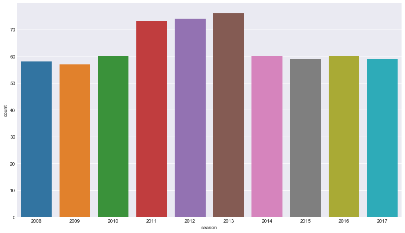
Which season had most number of matches?
We know that if each row is a match, then counting the number of instances/rows of every season would give us the number of matches for every season.
sns.countplot(x='season', data=matches)
plt.show()
countplot() function in seaborn does the job right away (without the need of an explicit group_by and count)
Gives this:
The most successful IPL Team
The most successful IPL team is the team that has won most number of times. Which also means, answer it to this is as same as the above exercise except counting the number of instances in each season, here we’ve to count the number of instances in each winning team.
#sns.countplot(y='winner', data = matches)
#plt.show
data = matches.winner.value_counts()
sns.barplot(y = data.index, x = data, orient='h');
Gives this:
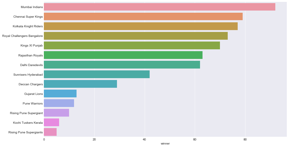
While this also could’ve been easily done with countplot(), just to introduce another variant of sns plot -barplot() has been used to visualize it.
Top player of the match Winners
top_players = matches.player_of_match.value_counts()[:10]
#sns.barplot(x="day", y="total_bill", data=tips)
fig, ax = plt.subplots()
ax.set_ylim([0,20])
ax.set_ylabel("Count")
ax.set_title("Top player of the match Winners")
#top_players.plot.bar()
sns.barplot(x = top_players.index, y = top_players, orient='v'); #palette="Blues");
plt.show()
Gives this:
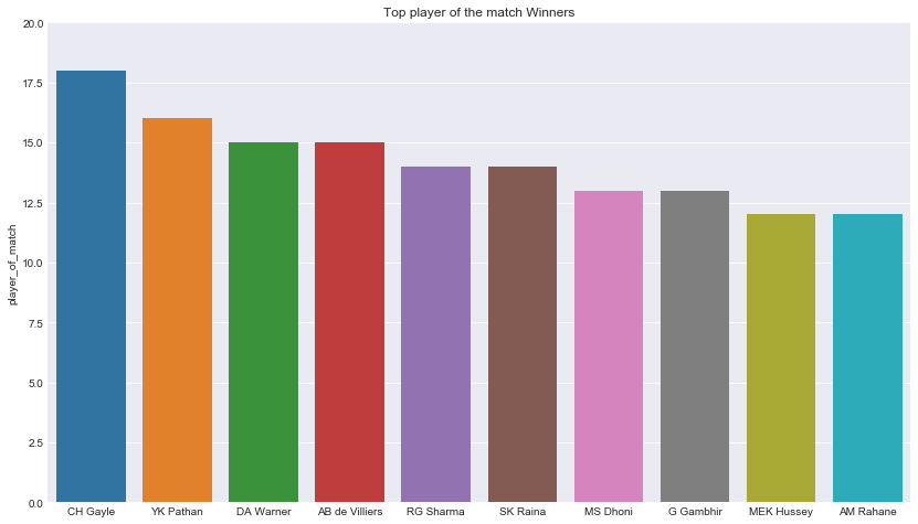
For those who follow IPL, you might have been wondering the irony now. Chris Gayle, is the most successful IPL player, wasn’t sold in the first round.
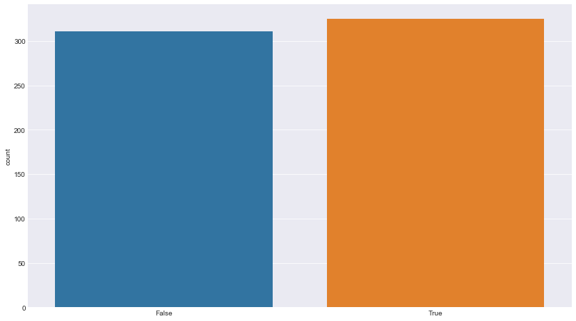
Has Toss-winning helped in Match-winning?
Having solved those not-so-tough questions above, we are nowhere to extract a critical insight – which is – Has winning toss actually helped in winning the match?
Using our same approach of dividing our problem into chunks – we can separate this question into two – match winner and toss winner if both of them are same – then it’s a success and if not it’s a failure. Before visualizing the outcome, let us first see how the numbers look.
ss = matches['toss_winner'] == matches['winner']
ss.groupby(ss).size()
False    311
True     325
dtype: int64
Looks like, Toss winning actually helps in Match winning – or to be statistically right, we could say there’s a correlation between Toss Winning and Match Winning and so we can assume that it helps.
To visualize the result:
#sns.countplot(matches['toss_winner'] == matches['winner'])
sns.countplot(ss);
Gives this plot:
With that, we’ve come to the end of this tutorial and as you might have noticed, It just took one line to almost many of the above questions to answers. That tells us two things: Python Expressions are very crispy in terms of its syntax and the second thing is, It doesn’t need to be tens and hundreds of line to bring out a valuable insight – just a few lines could do the magic – If you’re asking the right question!
Hope this post helps you in starting your journey of Data Analysis in Python. If you are interested in knowing more, Check out this free Intro to Python for Data Science Course. The complete code used here is available on my github.