Financial time series analysis and their forecasting have an history of remarkable contributions. It is then quite hard for the beginner to get oriented and capitalize from reading such scientific literature as it requires a solid understanding of basic statistics, a detailed study of the ground basis of time series analysis tools and the knowledge of specific statistical models used for financial products. Further, the financial time series ecosystem is not one of the most easiest flavour you may encounter. Trends are typically transitory as driven by underlying random processes, non stationarity, heteroscedasticity, structural breaks and outliers are rather common. All that has driven the adoption of sophisticated models and simulation techniques which require good understanding and expertise to take advantage of.
On the other hand, you may want to get a basic understanding of stock prices time series forecasting by taking advantage of a simple model providing with a sufficient reliability. For such purpose, the Black-Scholes-Merton model as based upon the lognormal distribution hypothesis and largely used in financial analysis can be helpful. The rest of this short dissertation shows how to take advantage of it.
Model
As said, I am going to introduce the Black-Scholes-Merton model which assumes that percentage changes in the stock price in a short period of time are normally distributed.
The return of the stock price S(t) at time t can be expressed under those hypothesis as:
$$
\begin{equation}
\begin{aligned}
\frac{S(t)-S(t_{0})}{S(t_{0})}\ \sim\ N(u\ \Delta T,\ \sigma^2\Delta T) \ \ \ \ \ (1) \\
\end{aligned}
\end{equation}
$$
where the left term is the (discrete) return on stock price S at time t. By formulating the same equation in terms of first order differentials for price S (dS) and time t (dt), the equation (1) turns out to be expressed in terms of continuously compounded returns, obtaining:
$$
\begin{equation}
\begin{cases}
t = t_{0} + \Delta T \\
ln(\frac{S(t)}{S(t_{0})})\ \sim \ N((u\ -\ \frac{\sigma^2}{2})\ \Delta T,\ \sigma^2\Delta T) \ \ \ \ \ (2) \\
\end{cases}
\end{equation}
$$
Equation (2) states that the log returns follow a normal distribution, where u is the stock price drift, σ is the stock price standard deviation. From equation (2), it can be stated the following relationship binding stock price S(t) with stock price S(t0):
$$
\begin{equation}
\begin{aligned}
S(t)\ =\ S(t_{0})\ e^{(u\ -\ \frac{\sigma^2}{2})\ +\ \sigma B(t)} \ \ \ \ \ (3) \\
\end{aligned}
\end{equation}
$$
The B(t) term represents the Brownian motion.
Furthermore, equation (2) allows to determine the distribution of the stock price as stated by the following equation:
$$
\begin{equation}
\begin{aligned}
\ln(S(t_{0}+\Delta T))\ \sim \ N(ln(S(t_{0})) + (u\ -\ \frac{\sigma^2}{2})\Delta T,\ \sigma^2\Delta T)\ \ \ \ \ (4) \\
\end{aligned}
\end{equation}
$$
The drift u and the standard deviation σ can be estimated from the stock price time series history.
The time interval ΔT represents our future horizon. Please note that both the drift and the standard deviation must refer to the same time scale, in the sense that if ΔT is measured in days, we have to use the daily returns and daily standard deviation, if ΔT is measured in weeks, we have to use weekly returns and weekly standard deviation, and so on.
Taking the exponential of both terms of equation (4) we obtain:
$$
\begin{equation}
\begin{aligned}
S(t_{0} + \Delta T)\ \sim \ exp(\ N(ln(S(t_{0})) + (u\ -\ \frac{\sigma^2}{2})\ \Delta T,\ \sigma^2 \Delta T)) \\
= exp(\ N(\ \hat u(\Delta T),\ \hat\sigma^2(\Delta T)) \ \ \ \ \ (5) \\
\end{aligned}
\end{equation}
$$
Above equation provides with a family of normal distributions having known parameters and dependent on the time interval ΔT = [0, T]. Lower and upper bounds at each instant of time t in ΔT can be modeled as a 95% confidence interval as determined by the 1.96 multiple of the standard deviation at time t in ΔT. As a result, the expected value, lower and upper bounds of the stock price S(t) are so determined:
$$
\begin{equation}
\begin{cases}
E(S(t))\ =\ exp(ln(S(t_{0})) + (u\ -\ \frac{\sigma^2}{2})\ \Delta T) \ \ \ \ \ (6) \\
LB(S(t))\ = exp(ln(S(t_{0})) + (u\ -\ \frac{\sigma^2}{2})\ \Delta T\ -\ 1.96*\sigma \sqrt \Delta T) \\
UB(S(t))\ = exp(ln(S(t_{0})) + (u\ -\ \frac{\sigma^2}{2})\ \Delta T\ +\ 1.96*\sigma \sqrt \Delta T) \\
\end{cases}
\end{equation}
$$
Implementation
I will take advantage of the timeSeries package for computing returns (see returns() function) and the quantmod package for financial stock prices availability (see getSymbols() function). Specifically, I will download the Apple share price history.
suppressPackageStartupMessages(library(timeSeries))
suppressPackageStartupMessages(library(quantmod))

# downloading stock price
getSymbols("AAPL")

head(AAPL)
           AAPL.Open AAPL.High AAPL.Low AAPL.Close AAPL.Volume AAPL.Adjusted
2007-01-03     86.29     86.58    81.90      83.80   309579900      10.85709
2007-01-04     84.05     85.95    83.82      85.66   211815100      11.09807
2007-01-05     85.77     86.20    84.40      85.05   208685400      11.01904
2007-01-08     85.96     86.53    85.28      85.47   199276700      11.07345
2007-01-09     86.45     92.98    85.15      92.57   837324600      11.99333
2007-01-10     94.75     97.80    93.45      97.00   738220000      12.56728
# using adjusted close price
Y <- coredata(AAPL[,"AAPL.Adjusted"])

# history time span
hist_start <- 1
hist_end <- 100
hist <- c(hist_start:hist_end)

# historical prices
Y.hist <- Y[hist]

# historical returns = (Y(t1)-Y(t0))/Y(t0)
Y.hist.ret <- returns(Y.hist)

# standard deviation computed based on history
(sv_hist <- sd(Y.hist.ret, na.rm=T))
[1] 0.01886924
Aboveshown value is the estimate of our standard deviation of our share price daily returns as determined by hystorical observations.
It is a good practice to compute the confidence intervals for estimated parameters in order to understand if we have sufficient precision as implied by the samples set size.
# 95% confidence interval
n <- length(hist)
sv_hist_low <- sqrt((n-1)*sv_hist^2/qchisq(.975, df=n-1))
sv_hist_up <- sqrt((n-1)*sv_hist^2/qchisq(.025, df=n-1))
(sv_hist_confint_95 <- c(sv_hist_low, sv_hist, sv_hist_up))
[1] 0.01656732 0.01886924 0.02191993
I am going to show a plot outlining future share price evolution.
# relative future time horizon
t <- 1:20

# martingale hypothesis (the average of future returns is equal to the current value)
u <- 0

# future expected value as based on normal distribution hypothesis
fc <- log(Y.hist[hist_end]) + (u - 0.5*sv_hist^2)*t

# lower bound 95% confidence interval
fc.lb <- fc - 1.96*sv_hist*sqrt(t)

# upper bound 95% confidence interval
fc.ub <- fc + 1.96*sv_hist*sqrt(t)

# collecting lower, expected and upper values
fc_band <- list(lb = exp(fc.lb), m = exp(fc), ub = exp(fc.ub))

# absolute future time horizon
xt <- c(hist_end + t)

# stock price history line plot
plot(Y[hist_start:(hist_end + max(t))], type='l',
     xlim = c(0, hist_end + max(t)),
     ylim = c(5, 20),
     xlab = "Time Index",
     ylab = "Share Price",
     panel.first = grid())
# starting point for our forecast
suppressWarnings(points(x = hist_end, y = Y.hist[hist_start+hist_end-1], pch = 21, bg = "green"))
# lower bound stock price forecast
lines(x = xt, y = fc_band$lb, lty = 'dotted', col = 'violet', lwd = 2)
# expected stock price forecast
lines(x = xt, y = fc_band$m, lty = 'dotted', col = 'blue', lwd = 2)
# upper bound stock price forecast
lines(x = xt, y = fc_band$ub, lty = 'dotted', col = 'red', lwd = 2)
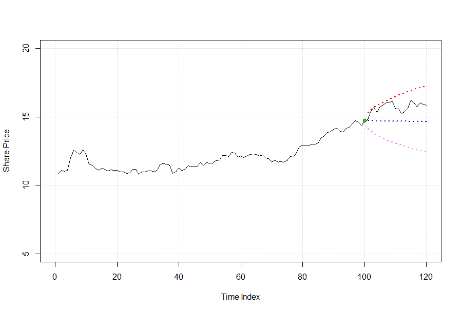
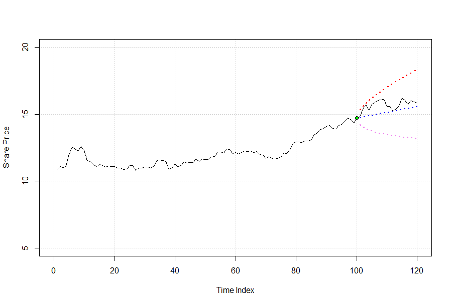
The plot shows the lower (violet) and upper (red) bounds including the actual future price evolution and the forecasted expected value (blue). In that, I did not account for a drift u (u = 0) and as a consequence, there is a flat line representing the future expected value (actually its slope is slightly negative as determined by the -0.5*σ^2 term).
If you like to have future stock price drift more consistent with its recent history, you may compute a return based on the same time scale of the standard deviation.
The lines of code to add are the following:
# added line of code
(mu_hist <- mean(Y.hist.ret, na.rm=T))

n <- length(hist)
# 95% confidence interval for the mean
mu_hist_low <- mu_hist - qt(0.975, df=n-1)*sv_hist/sqrt(n)
mu_hist_up <- mu_hist + qt(0.975, df=n-1)*sv_hist/sqrt(n)
(mu_hist_confint_95 <- c(mu_hist_low, mu_hist, mu_hist_up))
[1] -0.0006690514  0.0030750148  0.0068190811
Above the confidence interval for historical daily returns is shown. We have also to change the assigment to the variable u, the drift.
# drift computed on historical values
(u <- mu_hist)
[1] 0.0030750148
Furthermore, the code shown above can be easily enhanced with sliders to specify the stock price history to take into account for parameters estimation and the desired future time horizon. That can be done by taking advantage of the manipulate package or by implementing a Shiny gadget or application, for example.
Using the same model is possible to compute the probability that the future stock price be above or below a predetermined value at time t. That is possible by computing the normal distribution parameters as a function of ΔT = t – t0 and a density distribution basic property. Herein is how.
This is the historical share price daily drift u:
(u <- mu_hist)
[1] 0.003075015
This is the current share price S(t0):
(curr_share_price <- Y.hist[hist_end])
[1] 14.72056
This is the mean mu_t of our normal distribution computed with ΔT= 10, ten units of time (days) ahead of the current time:
t <- 10
(mu_t <- log(curr_share_price) + u - 0.5*sv_hist^2)*t
[1] 26.92142
This is the standard deviation sv_t of our normal distribution computed with ΔT = 10, ten units of time (days) ahead of the current time:
(sv_t <- sv_hist*sqrt(t))
[1] 0.05966977
Arbitrarly, I determine a target price 10% higher of the current one and hence equal to:
(target_share_price <- 1.10*curr_share_price)
[1] 16.19261
The probability that the share price at time t is equal or greater (please note the lower.tail = FALSE parameter) than the target price is the following:
pnorm(q = log(target_share_price),
      mean = mu_t,
      sd = sv_t,
      lower.tail = FALSE)
[1] 0.06072166
Our model states there is a probability of 6% that share price is above or equal to the target price.
The Misbehavior of Markets: criticism to the lognormal hypothesis
In 1963, Mandelbrot published a research highlighting that, contrary to the general assumption that share price movements were normally distributed, they instead followed a Pareto-Levy distribution, which has infinite variance. That implies that values considered with negligible probability determined by normal distribution hypothesis, they actually are not that unlikely to happen in case of Pareto-Levy distribution.
Based on that market booms and crashes are more frequent than we may think. Be aware of this while applying lognormal distribution assumptions.
Conclusions
We have outlined an approach that can be easily implemented to compute expected values, lower and upper bounds of future stock prices. That is based on the well known Black-Scholes-Merton model and its normal distribution hypothesis.
The plot showing future share price expected value, lower and upper bounds can be enhanced with interactive inputs to allow users to select history length and future horizon of interest. By using the same model, probabilities associated to future price thresholds can be computed.
A reference for the Black-Scholes-Merton model we talked about can be found in the following book:
- Options, Futures and Other Derivatives, John C. Hull, Prentice Hall, 8th Ed.
A reference for Mandlebrot criticism to share price lognormal distribution hypothesis is the following book:
- The Misbehavior of Markets: a Fractal View of Finance Turbolence, Benoit Mandelbrot & Richard L. Hudson, Basic Books Ed.
Disclaimer
Any securities or databases referred in this post are solely for illustration purposes, and under no regard should the findings presented here be interpreted as investment advice or a promotion of any particular security or source.
If you have any question, feel free to comment below.

