Dummy Variable for Examining Structural Instability in Regression: An Alternative to Chow Test

One of the fast-growing economies in the era of globalization is the Ethiopian economy. Among the lower-income group countries, it has emerged as one of the rare countries to achieve a double-digit growth rate in Gross Domestic Product (GDP). However, there is a great deal of debate regarding the double-digit growth rate, especially during the recent global recession period. So, it becomes a question of empirical research whether there is a structural change in the relationship between the GDP of Ethiopia and the regressor (time).

How do we find out that a structural change has in fact occurred? To answer this question, we consider the GDP of Ethiopia (measured on constant 2010 US$) over the period of 1981 to 2015. Like many other countries in the world, Ethiopia has adopted the policy of regulated globalization during the early nineties of the last century. So, our aim is to whether the GDP of Ethiopia has undergone any structural changes following the major policy shift due to adoption of globalization policy. To answer this question, we have two options in statistical and econometric research. The most important classes of tests on structural change are the tests from the generalized fluctuation test framework (Kuan and Hornik, 1995) on the one hand and tests based on F statistics (Hansen, 1992; Andrews, 1993; Andrews and Ploberger, 1994) on the other. “The first class includes, in particular, the CUSUM and MOSUM tests and the fluctuation test, while the Chow and the supF test belong to the latter. A topic that gained more interest rather recently is to monitor structural change, i.e., to start after a history phase (without structural changes) to analyze new observations and to be able to detect a structural change as soon after its occurrence as possible” (Zeileis, Leisch, Hornik and Kleiber, 2002).

Let us divide the whole study period in two sub-periods

1. pre-globalization (1981 – 1991)
2. post-globalization (1992-2015)

$$\text {Pre – globalization period (1981 – 1991):} ~~~ lnGDP=\beta_{01} +β_{11} t +u_1 \\ \text {Post – globalization period (1992 – 2015):}~~~ lnGDP=\beta_{02} +\beta_{12} t+u_2 \\ \text {Whole period (1981 – 2015):} ~~~ lnGDP=\beta_0 +\beta_1 t +u$$

The regression for the whole period assumes that there is no difference between the two time periods and, therefore, estimates the GDP growth rate for the entire time period. In other words, this regression assumes that the intercept, as well as the slope coefficient, remains the same over the entire period; that is, there is no structural change. If this is, in fact, the situation, then
$\beta_{01} =\beta_{02}=\beta_0 ~~~~and~~~~ \beta_{11} =\beta_{12} =\beta_1$

The first two regression lines assume that the regression parameters are different in two sub-period periods, that is, there is structural instability either because of changes in slope parameters or intercept parameters.

Solution by Chow

To apply Chow test to visualize the structural changes empirically, the following assumptions are required:

i. The error terms for the two sub-period regressions are normally distributed with the same variance;
ii. The two error terms are independently distributed.
iii. The break-point at which the structural stability to be examined should be known apriori.

The Chow test examines the following set of hypotheses:
$$H_0 : \text {There is no structural change} \\ against \\ H_1 : \text {There is a structural change}$$

Steps in Chow test

Step 1: Estimate third regression assuming that there is no parameter instability, and obtain the Residual Sum Squares $RSS_R ~~ with ~~~df =(n_1 +n_2−2k ) \\ where~~k=\text {No of parameters estimated}\\ n_1= \text {No of observations in first period}\\n_2=\text {No of observations in second sub-periods}$
So, in present case $k = 2,$ as there are two parameters (intercept term and slope coefficient).

We call this Restricted Residual Sum Squares as it assumes the restriction of structural stability, that is, $\beta_{01}=\beta_{02}=\beta_{0} ~~~and~~~\beta_{11}=\beta_{12}=\beta_1$

Step 2: Estimate the first and second regressions assuming that there is parameter instability and obtain the respective Residual Sum Squares as
$RSS_1 = \text {Residual Sum Squares for the first sub-period regression with}~~ df =n_1−k \\RSS_2 = \text {Residual Sum Squares for the second sub-period regression with}~~ df =n_2−k$

Step 3: As the two sets of samples supposed to be independent, we can add $RSS_1$ and $RSS_2$ and the resultant Residual Sum Squares may be called the Unrestricted Residual Sum of Squares, that is, $RSS_{UR}=RSS_1 + RSS_2 ~~~with ~~~df = (n_1 + n_2 -2k)$
The test statistic to be used is given as:
$F= \frac {\left (RSS_R – RSS_{UR} \right)/k}{\left (RSS_{UR}\right)/(n_1 +n_2 -2k)}$

Under the assumption of true null hypothesis, this follows F-distribution.

Now if this F-test is significant, we can reject the null hypothesis of no structural instability and conclude that the fluctuations is the GGP is high enough to believe that it leads to structural instability in the GDP growth path.

Importing the Data into R

Importing the data saved in csv format gdp_ethiopia

gdp<-read.csv(file.choose(), sep = ",", header = TRUE)
attach(gdp)
gdp$lGDP<-log(GDP)
attach(gdp)
Copy

Let us have a look at the scatter plot of GDP against time using ggplot2 package

library(ggplot2)
ggplot(gdp, aes(YEAR,GDP)) +
   geom_line(col="red") +
   labs(title="GDP Growth of Ethiopia")
Copy

Gives this plot:

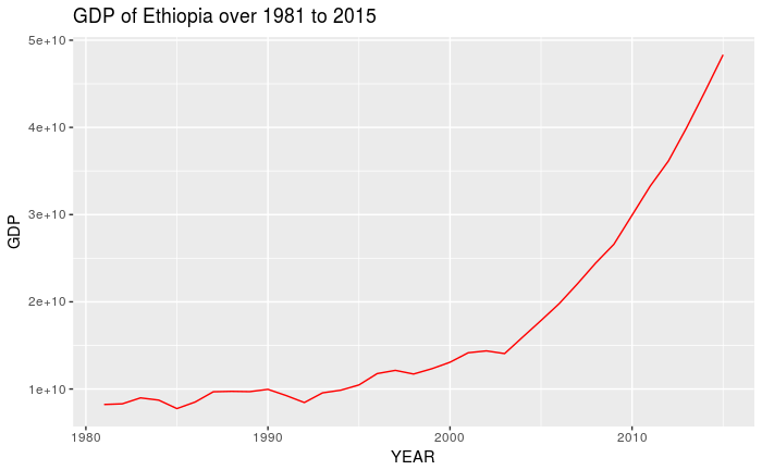
As observed from the figure that the growth of GDP gets momentum after the adoption of the new policy regime, especially after 2000. Until 1992-93, the economy was looking as a stagnant as the GDP curve was more or less parallel to the x-axis. It is only after 1993 that the GDP started to grow and the growth became more prominent after 2000. To confirm this, we will apply the Chow test by considering the break-point in the year 1992 when the new economic policy was adopted by the Ethiopian government.
To fit the model of GDP growth path by assuming that there is no structural instability in the model, we need to create the time variable by using the following code to do so:

gdp$t<-seq(1:35)
Copy

For estimating the growth of GDP for the whole period

model0<-lm(lGDP~t, data = gdp)
summary(model0)
Call:
lm(formula = log(GDP) ~ t, data = ethio_gdp)

Residuals:
     Min       1Q   Median       3Q      Max 
-0.28379 -0.17673  0.01783  0.16134  0.34789 

Coefficients:
             Estimate Std. Error t value Pr(>|t|)    
(Intercept) 22.495383   0.066477   338.4   <2e-16 ***
t            0.050230   0.003221    15.6   <2e-16 ***
---
Signif. codes:  0 ‘***’ 0.001 ‘**’ 0.01 ‘*’ 0.05 ‘.’ 0.1 ‘ ’ 1

Residual standard error: 0.1924 on 33 degrees of freedom
Multiple R-squared:  0.8805,	Adjusted R-squared:  0.8769 
F-statistic: 243.2 on 1 and 33 DF,  p-value: < 2.2e-16


Copy

Thus, we see that over the entire period, the GDP is growing at an annual growth rate of 5 percent.
We’ll use this object ‘model0’ to apply Chow test in R. For this, we need to load the package called ‘strucchange’ by using the following code:

library(strucchange)
Copy

The break-point occurs in 1992 which will coincide with 12 in sequence 1 to 35 corresponding to the year 1981 to 2015. The code and results are shown below:

sctest(lGDP~t, type = "Chow", point = 12)
Chow test
			data:  log(gdp_ethio) ~ t
			F = 51.331, p-value = 1.455e-10

Copy

The above result shows that the F-value is 51.331 and the corresponding p-value is much less than the level of significance (0.05) implying that the test is significant. This confirms that there is structural instability in the GDP growth path of Ethiopia at the break-point 1992.
However, we cannot tell whether the difference in the two regressions is because of differences in the intercept terms or the slope coefficients or both. Very often this knowledge itself is very useful. For analyzing such a situation, we have the following four possibilities:
I. Coincident Regression where both the intercept and the slope coefficients are the same in the two sub-period regressions;
II. Parallel Regression where only the intercepts in the two regressions are different but the slopes are the same;
III. Concurrent Regression where the intercepts in the two regressions are the same, but the slopes are different; and
IV. Dis-similar Regression where both the intercepts and slopes in the two regressions are different.
Let us examine case by case.

II. Parallel Regression where only the intercepts in the two regressions are different but the slopes are the same

Suppose the economic reforms do not influence the slope parameter but instead simply affect the intercept term.
Following the economic reforms in 1992, we have the following regression models in two sub-periods – pre-globalization (1981 – 1991) and post-globalization (1992-2015).
$\begin {aligned} \text {Pre-globalization (1981 – 1991):}~~~& lnGDP=β_{01} +β_{11} t +u_1\\ \text {Post – globalization period (1992 – 2015):}~~~& lnGDP=β_{02} +β_{12} t+u_2\\ \text {Whole period (1981 – 2015):}~~~& lnGDP=β_0 +β_1 t +u \end {aligned}$

If there is no structural change:

$\beta_{01}=\beta_{02}=\beta_0 \\and \\ \beta_{11}=\beta_{12}=\beta_1$

If there is structural change and that affects only the intercept terms, not the slope coefficients, we have:

$\beta_{01}\ne\beta_{02}\\and \\ \beta_{11}=\beta_{12}$

To capture this effect, the dummy variable $D$ is included in the following manner:

$\begin {aligned} lGDP&=\beta_0+\beta_1 t+\beta_2 D+u\\where~~D&=1~~\text {for the post-reform period (sub-period 2)} \\ &=0~~ \text {for the post-reform period (sub-period 2)} \end {aligned}$

The difference in the logarithm of GDP between the two sub-periods is given by the coefficient $\beta_2$.

If $D = 1$, then for the post-reform period, $\widehat {lGDP} = \hat\beta_0+\hat\beta_1 t+\hat\beta_2$

If $D=0,$ then for the pre-reform period, $\widehat {lGDP} = \hat\beta_0+\hat\beta_1 t$

Using the ‘gdp_ethiopia.csv’ data-file, this model can be estimated. The R code along with the explanation is produced below:

gdp$D=1992,1,0) 
attach(gdp)
gdp$D<-factor(D, levels = c(0,1), labels = c("pre","post"))
attach(gdp)
model1<-lm(lGDP~t+D, data = gdp)
summary(model1)
Call:
lm(formula = lGDP ~ t + D, data = gdp)

Residuals:
      Min        1Q    Median        3Q       Max 
-0.309808 -0.080889  0.006459  0.087419  0.257020 

Coefficients:
             Estimate Std. Error t value Pr(>|t|)    
(Intercept) 22.505310   0.046417 484.847  < 2e-16 ***
t            0.068431   0.003783  18.089  < 2e-16 ***
Dpost       -0.492244   0.082302  -5.981 1.15e-06 ***
---
Signif. codes:  0 ‘***’ 0.001 ‘**’ 0.01 ‘*’ 0.05 ‘.’ 0.1 ‘ ’ 1

Residual standard error: 0.1343 on 32 degrees of freedom
Multiple R-squared:  0.9436,	Adjusted R-squared:  0.9401 
F-statistic: 267.6 on 2 and 32 DF,  p-value: < 2.2e-16

Copy

So, the estimated regression model is given by
$\widehat {lGDP}= 22.505+0.068t-0.492D$

This would imply that
For the post-reform period: $$\widehat {lGDP}= 22.013+0.068t$$

For the pre-reform period: $$\widehat {lGDP}= 22.505+0.068t$$

To graphically visualize this, use the following code to produce the following graphs:

gdp<-cbind(gdp, pred=predict(model1))
library(ggplot2)
ggplot(data=gdp, mapping=aes(x=t, y=lGDP, color=D)) + geom_point() + geom_line(mapping=aes(y=pred))
Copy

Gives this plot:

III. Concurrent Regression where the intercepts in the two regressions are the same, but the slopes are different

Now we assume that the economic reforms do not influence the intercept term $\beta_0$, but simply affect the slope parameter. That is, in terms of our present example, we can say that
$β_{01} =β_{02} \\and\\ β_{11} \ne β_{12}$

To capture the effects of such changes in slope parameters, it is necessary to add the product of time-variable $t$ and the dummy variable $D$. The new variable $tD$ is called the interaction variable or slope dummy variable since it allows for a change in the slope of the relationship.

The modified growth estimation model is:

$lGDP=\beta_0 +\beta_1t+\beta_2 tD+u$
Obviously, when $D = 1,$ then $\widehat{lGDP}=\hat\beta_0 +\hat\beta_1t+\hat\beta_2 t \\\implies \widehat{lGDP}=\hat\beta_0 +(\hat\beta_1+\hat\beta_2)t$

when $D=0$, then $\widehat{lGDP}=\hat\beta_0+\hat\beta_1t$

The necessary R codes and the results are produced below:

attach(gdp)
gdp$D1=1992,1,0)
attach(gdp)
gdp$tD<-t*D1
attach(gdp)
model2<-lm(lGDP~t+tD,data = gdp)
summary(model2)
Call:
lm(formula = lGDP ~ t + tD, data = gdp)

Residuals:
     Min       1Q   Median       3Q      Max 
-0.26778 -0.14726 -0.04489  0.13919  0.35627 

Coefficients:
            Estimate Std. Error t value Pr(>|t|)    
(Intercept) 22.40377    0.09125 245.521  < 2e-16 ***
t            0.07072    0.01458   4.851 3.06e-05 ***
tD          -0.01721    0.01195  -1.440     0.16    
---
Signif. codes:  0 ‘***’ 0.001 ‘**’ 0.01 ‘*’ 0.05 ‘.’ 0.1 ‘ ’ 1

Residual standard error: 0.1894 on 32 degrees of freedom
Multiple R-squared:  0.8878,	Adjusted R-squared:  0.8808 
F-statistic: 126.6 on 2 and 32 DF,  p-value: 6.305e-16

Copy

In the above results, it is evident that the interaction term (tD) is not statistically significant as the corresponding p-value is much higher than the level of significance (5% or 0.05). This would imply that the economic reforms do not affect the slope term. However, for visualizing the results graphically we proceed as follows:
The estimated regression model is:
$\widehat {lGDP} = 22.404+0.071t-0.017tD$
This would imply the following growth functions for both the periods.
$\widehat {lGDP} = 22.404+0.054t~~~~~~\text {for the post-reform period}\\ \widehat {lGDP} = 22.404+0.071t~~~~~~\text {for the pre-reform period}$

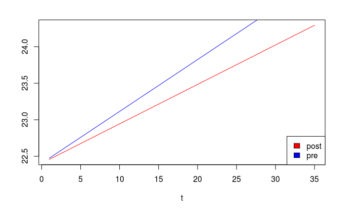
Notice that the slope, rather than the intercept of the growth function changed. This can graphically shown below:

curve((22.404+0.054*x), xlab = "t", ylab = "", xlim = c(1,35), col="red")
curve(22.404+0.071*x, xlab = "t", ylab = "", xlim = c(1,35), col="blue", add = TRUE)
legend( "bottomright", legend = c("post", "pre"), fill = c("red", "blue") )
Copy

Gives this plot:

IV. Dis-similar Regression (both the intercepts and slopes are different)

In this case, both the intercept and the slope of the growth function changed simultaneously. The statistical model to capture such changes can be represented by the following equation.
The modified statistical model to capture such changes can be represented by the following equation.

$lGDP=\beta_0 +\beta_1 t +\beta_2 D+\beta_3 tD+u$

Obviously, when $D=1$, then for the post-reform period: $\widehat{lGDP}=\hat\beta_0 +\hat\beta_1 t+\hat\beta_2 +\hat\beta_3 t +u \\=(\hat\beta_0 +\hat\beta_2 )+(\hat\beta_1 + \hat\beta_3) t +u$

when $D=0$, then for the pre-reform period: $\widehat{lGDP}= \hat\beta_0 + \hat\beta_1 t +u$
The model is estimated using the following codes and the results are produced below:

model3<-lm(lGDP~t+D+t*D, data = gdp)
summary(model3)
Call:
lm(formula = lGDP ~ t + D + t * D, data = gdp)

Residuals:
     Min       1Q   Median       3Q      Max 
-0.21768 -0.05914  0.01033  0.07033  0.13777 

Coefficients:
             Estimate Std. Error t value Pr(>|t|)    
(Intercept) 22.807568   0.060484 377.084  < 2e-16 ***
t            0.018055   0.008918   2.025   0.0516 .  
Dpost       -0.907739   0.090685 -10.010 3.13e-11 ***
t:Dpost      0.055195   0.009335   5.913 1.57e-06 ***
---
Signif. codes:  0 ‘***’ 0.001 ‘**’ 0.01 ‘*’ 0.05 ‘.’ 0.1 ‘ ’ 1

Residual standard error: 0.09353 on 31 degrees of freedom
Multiple R-squared:  0.9735,	Adjusted R-squared:  0.9709 
F-statistic: 379.4 on 3 and 31 DF,  p-value: < 2.2e-16

Copy

Thus, our estimated regression model is written as:
$\widehat {lGDP} = 22.808 + 0.018 t -0.908 D +0.0552 tD$

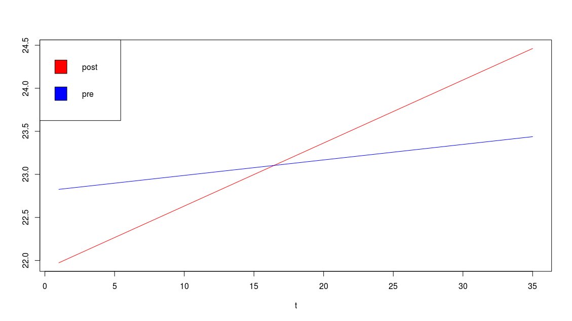
$\widehat {lGDP} = 21.9+0.0732t~~~~~~\text {for the post-reform period}\\ \widehat {lGDP} = 22.808+0.018t~~~~~~\text {for the pre-reform period}$

To visualize the matter, the following codes are used to produce the figure below.

curve(21.9+0.0732*x, xlab = "t", ylab = "", xlim = c(1,35), col="red")
curve(22.808+0.018*x, xlab = "t", ylab = "", xlim = c(1,35), col="blue", add = TRUE)
legend( "topleft", legend = c("post", "pre"), fill = c("red","blue") )
Copy

Gives this plot:

That’s all. If you have questions, post comments below. The R script for the estimation of the whole analysis is rcode.