Splines are a smooth and flexible way of fitting Non linear Models and learning the Non linear interactions from the data.In most of the methods in which we fit Non linear Models to data and learn Non linearities is by transforming the data or the variables by applying a Non linear transformation.
Cubic Splines
Cubic Splines with knots(cutpoints) at \(\xi_K , \ K = 1,\ 2…\ k\) is a piece-wise cubic polynomial with continious derivatives upto order 2 at each knot. They have continuous 1st and 2nd derivative. The order of continuity is = \( (d – 1) \) , where \(d\) is the degree of polynomial. Now we can represent the Model with truncated power Basis function \(b(x)\). What happens is that we transform the variables \(X_i\) by applying a Basis function \(b(x)\) and fit a model using these transformed variables which adds non linearities to the model and enables the splines to fit smoother and flexible Non linear functions.
The Regression Equation Becomes —
\(f(x) = y_i = \alpha + \beta_1.b_1(x_i)\ + \beta_2.b_2(x_i)\ + \ …. \beta_{k+3}.b_{k+3}(x_i) \ + \epsilon_i\)
#loading the Splines Packages
require(splines)
#ISLR contains the Dataset
require(ISLR)
attach(Wage) #attaching Wage dataset
?Wage #for more details on the dataset
agelims<-range(age)
#Generating Test Data
age.grid<-seq(from=agelims[1], to = agelims[2])
Now let’s fit a Cubic Spline with 3 Knots (cutpoints)
The idea here is to transform the variables and add a linear combination of the variables using the Basis power function to the regression function f(x).The \( bs() \) function is used in R to fit a Cubic Spline.
#3 cutpoints at ages 25 ,50 ,60
fit<-lm(wage ~ bs(age,knots = c(25,40,60)),data = Wage )
summary(fit)
##
## Call:
## lm(formula = wage ~ bs(age, knots = c(25, 40, 60)), data = Wage)
##
## Residuals:
##     Min      1Q  Median      3Q     Max
## -98.832 -24.537  -5.049  15.209 203.207
##
## Coefficients:
##                                 Estimate Std. Error t value Pr(>|t|)
## (Intercept)                       60.494      9.460   6.394 1.86e-10 ***
## bs(age, knots = c(25, 40, 60))1    3.980     12.538   0.317 0.750899
## bs(age, knots = c(25, 40, 60))2   44.631      9.626   4.636 3.70e-06 ***
## bs(age, knots = c(25, 40, 60))3   62.839     10.755   5.843 5.69e-09 ***
## bs(age, knots = c(25, 40, 60))4   55.991     10.706   5.230 1.81e-07 ***
## bs(age, knots = c(25, 40, 60))5   50.688     14.402   3.520 0.000439 ***
## bs(age, knots = c(25, 40, 60))6   16.606     19.126   0.868 0.385338
## ---
## Signif. codes:  0 '***' 0.001 '**' 0.01 '*' 0.05 '.' 0.1 ' ' 1
##
## Residual standard error: 39.92 on 2993 degrees of freedom
## Multiple R-squared:  0.08642,    Adjusted R-squared:  0.08459
## F-statistic: 47.19 on 6 and 2993 DF,  p-value: < 2.2e-16
Now plotting the Regression Line
#Plotting the Regression Line to the scatterplot
plot(age,wage,col="grey",xlab="Age",ylab="Wages")
points(age.grid,predict(fit,newdata = list(age=age.grid)),col="darkgreen",lwd=2,type="l")
#adding cutpoints
abline(v=c(25,40,60),lty=2,col="darkgreen")
Gives this plot:
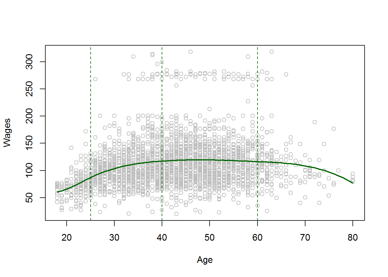
The Dashed Lines are the Cutpoints or the Knots. The above Plot shows the smoothing and local effect of Cubic Splines.
Smoothing Splines
These are mathematically more challenging but they are more smoother and flexible as well. But, it does not require the selection of the number of Knots, but require selection of only a Roughness Penalty which accounts for the wiggliness(fluctuations) and controls the roughness of the function and variance of the Model. Another important thing to remember in Smoothing Splines are that they have a Knot for every unique value of \((x_i)\).Our aim in Smoothing Splines is to minimize the Error function which is modified by adding a Roughness Penalty which penalizes it for Roughness(Wiggliness) and high variance.
\(minimize:{ g \in RSS} :\ \sum\limits_{i=1}^n ( \ y_i \ – \ g(x_i) \ )^2 + \lambda \ \int g”(t)^2 dt , \quad \lambda > 0\) .
\( \lambda \ is \ the \ Tuning \ Parameter \)
#fitting smoothing splines using smooth.spline(X,Y,df=...)
fit1<-smooth.spline(age,wage,df=16) #16 degrees of freedom
#Plotting both cubic and Smoothing Splines
plot(age,wage,col="grey",xlab="Age",ylab="Wages")
points(age.grid,predict(fit,newdata = list(age=age.grid)),col="darkgreen",lwd=2,type="l")
#adding cutpoints
abline(v=c(25,40,60),lty=2,col="darkgreen")
lines(fit1,col="red",lwd=2)
legend("topright",c("Smoothing Spline with 16 df","Cubic Spline"),col=c("red","darkgreen"),lwd=2)
Gives this plot:

Now as we can notice that the Red line i.e Smoothing Spline is more wiggly and fits data more flexibly.This is probably due to high degrees of freedom. The best way to select the value of \(\lambda\) and df is Cross Validation . Now we have a direct method to implement cross validation in R using smooth.spline().
Implementing Cross Validation to select value of λ and Implement Smoothing Splines:
fit2<-smooth.spline(age,wage,cv = TRUE)
fit2
## Call:
## smooth.spline(x = age, y = wage, cv = TRUE)
##
## Smoothing Parameter  spar= 0.6988943  lambda= 0.02792303 (12 iterations)
## Equivalent Degrees of Freedom (Df): 6.794596
## Penalized Criterion: 75215.9
## PRESS: 1593.383
#It selects $\lambda=0.0279$ and df = 6.794596 as it is a Heuristic and can take various values for how rough the #function is
plot(age,wage,col="grey")
#Plotting Regression Line
lines(fit2,lwd=2,col="purple")
legend("topright",("Smoothing Splines with 6.78 df selected by CV"),col="purple",lwd=2)
Gives this plot:
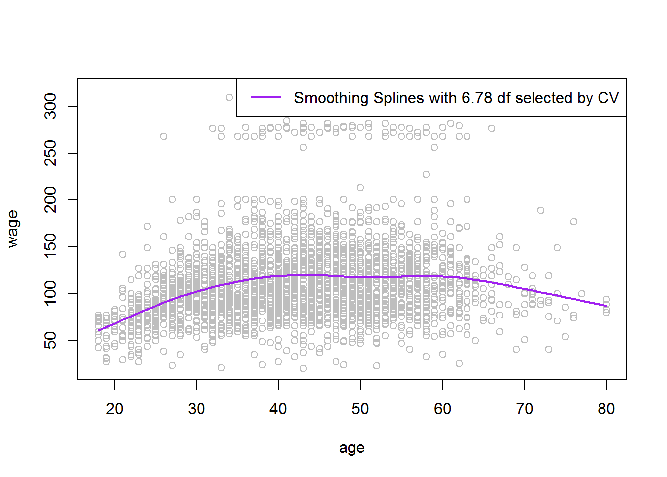
This Model is also very Smooth and Fits the data well.
Conclusion
Hence this was a simple overview of Cubic and Smoothing Splines and how they transform variables and add Non linearities to the Model and are more flexible and smoother than other techniques. It is better in terms of extrapolation and is more smoother.Other techniques such as Polynomial regression is very bad at extrapolation and oscillates a lot once it gets out of boundaries and it becomes very wiggly and fluctuating which shows the signs of High Variance and mostly Overfits at larger values of degree of polynomials. The main thing to remember while fitting Non linear Models to the data is that we need to do some transformations to data or the variables in order to make the model more flexible and stronger in learning Non linear Interactions between the Inputs \(X_i\) and Output \( Y \) variables.
Hope you guys liked the article and make sure to like and share it. Cheers!