Among the many R packages, there is the outbreaks package. It contains datasets on epidemics, on of which is from the 2013 outbreak of influenza A H7N9 in China, as analysed by Kucharski et al (2014). I will be using their data as an example to test whether we can use Machine Learning algorithms for predicting disease outcome.
To do so, I selected and extracted features from the raw data, including age, days between onset and outcome, gender, whether the patients were hospitalised, etc. Missing values were imputed and different model algorithms were used to predict outcome (death or recovery). The prediction accuracy, sensitivity and specificity. The thus prepared dataset was devided into training and testing subsets. The test subset contained all cases with an unknown outcome. Before I applied the models to the test data, I further split the training data into validation subsets.
The tested modeling algorithms were similarly successful at predicting the outcomes of the validation data. To decide on final classifications, I compared predictions from all models and defined the outcome “Death” or “Recovery” as a function of all models, whereas classifications with a low prediction probability were flagged as “uncertain”. Accounting for this uncertainty led to a 100% correct classification of the validation test set.
The training cases with unknown outcome were then classified based on the same algorithms. From 57 unknown cases, 14 were classified as “Recovery”, 10 as “Death” and 33 as uncertain.
The data
The dataset contains case ID, date of onset, date of hospitalisation, date of outcome, gender, age, province and of course the outcome: Death or Recovery. I can already see that there are a couple of missing values in the data, which I will deal with later.
# install and load package
if (!require("outbreaks")) install.packages("outbreaks")
library(outbreaks)
fluH7N9.china.2013_backup <- fluH7N9.china.2013 # back up original dataset in case something goes awry along the way
# convert ? to NAs
fluH7N9.china.2013$age[which(fluH7N9.china.2013$age == "?")] <- NA
# create a new column with case ID
fluH7N9.china.2013$case.ID <- paste("case", fluH7N9.china.2013$case.ID, sep = "_")
head(fluH7N9.china.2013)
## case.ID date.of.onset date.of.hospitalisation date.of.outcome outcome gender age province
## 1 case_1 2013-02-19 2013-03-04 Death m 87 Shanghai
## 2 case_2 2013-02-27 2013-03-03 2013-03-10 Death m 27 Shanghai
## 3 case_3 2013-03-09 2013-03-19 2013-04-09 Death f 35 Anhui
## 4 case_4 2013-03-19 2013-03-27 f 45 Jiangsu
## 5 case_5 2013-03-19 2013-03-30 2013-05-15 Recover f 48 Jiangsu
## 6 case_6 2013-03-21 2013-03-28 2013-04-26 Death f 32 Jiangsu Copy
Before I start preparing the data for Machine Learning, I want to get an idea of the distribution of the data points and their different variables by plotting. Most provinces have only a handful of cases, so I am combining them into the category “other” and keep only Jiangsu, Shanghai and Zhejian and separate provinces.
# gather for plotting with ggplot2
library(tidyr)
fluH7N9.china.2013_gather <- fluH7N9.china.2013 %>%
  gather(Group, Date, date.of.onset:date.of.outcome)

# rearrange group order
fluH7N9.china.2013_gather$Group <- factor(fluH7N9.china.2013_gather$Group, levels = c("date.of.onset", "date.of.hospitalisation", "date.of.outcome"))

# rename groups
library(plyr)
fluH7N9.china.2013_gather$Group <- mapvalues(fluH7N9.china.2013_gather$Group, from = c("date.of.onset", "date.of.hospitalisation", "date.of.outcome"),
          to = c("Date of onset", "Date of hospitalisation", "Date of outcome"))

# renaming provinces
fluH7N9.china.2013_gather$province <- mapvalues(fluH7N9.china.2013_gather$province,
                                                from = c("Anhui", "Beijing", "Fujian", "Guangdong", "Hebei", "Henan", "Hunan", "Jiangxi", "Shandong", "Taiwan"),
                                                to = rep("Other", 10))

# add a level for unknown gender
levels(fluH7N9.china.2013_gather$gender) <- c(levels(fluH7N9.china.2013_gather$gender), "unknown")
fluH7N9.china.2013_gather$gender[is.na(fluH7N9.china.2013_gather$gender)] <- "unknown"

# rearrange province order so that Other is the last
fluH7N9.china.2013_gather$province <- factor(fluH7N9.china.2013_gather$province, levels = c("Jiangsu",  "Shanghai", "Zhejiang", "Other"))

# convert age to numeric
fluH7N9.china.2013_gather$age <- as.numeric(as.character(fluH7N9.china.2013_gather$age))

library(ggplot2)
my_theme <- function(base_size = 12, base_family = "sans"){
  theme_minimal(base_size = base_size, base_family = base_family) +
  theme(
    axis.text = element_text(size = 12),
    axis.text.x = element_text(angle = 45, vjust = 0.5, hjust = 0.5),
    axis.title = element_text(size = 14),
    panel.grid.major = element_line(color = "grey"),
    panel.grid.minor = element_blank(),
    panel.background = element_rect(fill = "aliceblue"),
    strip.background = element_rect(fill = "lightgrey", color = "grey", size = 1),
    strip.text = element_text(face = "bold", size = 12, color = "black"),
    legend.position = "bottom",
    legend.justification = "top",
    legend.box = "horizontal",
    legend.box.background = element_rect(colour = "grey50"),
    legend.background = element_blank(),
    panel.border = element_rect(color = "grey", fill = NA, size = 0.5)
  )
}

# plotting raw data
ggplot(data = fluH7N9.china.2013_gather, aes(x = Date, y = age, fill = outcome)) +
  stat_density2d(aes(alpha = ..level..), geom = "polygon") +
  geom_jitter(aes(color = outcome, shape = gender), size = 1.5) +
  geom_rug(aes(color = outcome)) +
  labs(
    fill = "Outcome",
    color = "Outcome",
    alpha = "Level",
    shape = "Gender",
    x = "Date in 2013",
    y = "Age",
    title = "2013 Influenza A H7N9 cases in China",
    subtitle = "Dataset from 'outbreaks' package (Kucharski et al. 2014)",
    caption = ""
  ) +
  facet_grid(Group ~ province) +
  my_theme() +
  scale_shape_manual(values = c(15, 16, 17)) +
  scale_color_brewer(palette="Set1", na.value = "grey50") +
  scale_fill_brewer(palette="Set1")
Copy
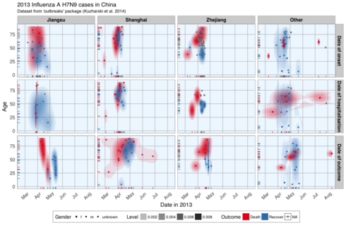
This plot shows the dates of onset, hospitalisation and outcome (if known) of each data point. Outcome is marked by color and age shown on the y-axis. Gender is marked by point shape. The density distribution of date by age for the cases seems to indicate that older people died more frequently in the Jiangsu and Zhejiang province than in Shanghai and in other provinces. When we look at the distribution of points along the time axis, it suggests that their might be a positive correlation between the likelihood of death and an early onset or early outcome.
I also want to know how many cases there are for each gender and province and compare the genders’ age distribution.
fluH7N9.china.2013_gather_2 <- fluH7N9.china.2013_gather[, -4] %>%
  gather(group_2, value, gender:province)

fluH7N9.china.2013_gather_2$value <- mapvalues(fluH7N9.china.2013_gather_2$value, from = c("m", "f", "unknown", "Other"),
          to = c("Male", "Female", "Unknown gender", "Other province"))

fluH7N9.china.2013_gather_2$value <- factor(fluH7N9.china.2013_gather_2$value,
                                            levels = c("Female", "Male", "Unknown gender", "Jiangsu", "Shanghai", "Zhejiang", "Other province"))

p1 <- ggplot(data = fluH7N9.china.2013_gather_2, aes(x = value, fill = outcome, color = outcome)) +
  geom_bar(position = "dodge", alpha = 0.7, size = 1) +
  my_theme() +
  scale_fill_brewer(palette="Set1", na.value = "grey50") +
  scale_color_brewer(palette="Set1", na.value = "grey50") +
  labs(
    color = "",
    fill = "",
    x = "",
    y = "Count",
    title = "2013 Influenza A H7N9 cases in China",
    subtitle = "Gender and Province numbers of flu cases",
    caption = ""
  )

p2 <- ggplot(data = fluH7N9.china.2013_gather, aes(x = age, fill = outcome, color = outcome)) +
  geom_density(alpha = 0.3, size = 1) +
  geom_rug() +
  scale_color_brewer(palette="Set1", na.value = "grey50") +
  scale_fill_brewer(palette="Set1", na.value = "grey50") +
  my_theme() +
  labs(
    color = "",
    fill = "",
    x = "Age",
    y = "Density",
    title = "",
    subtitle = "Age distribution of flu cases",
    caption = ""
  )

library(gridExtra)
library(grid)
grid.arrange(p1, p2, ncol = 2)Copy
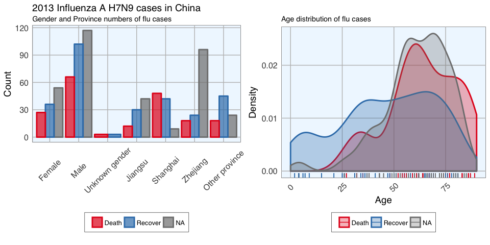
In the dataset, there are more male than female cases and correspondingly, we see more deaths, recoveries and unknown outcomes in men than in women. This is potentially a problem later on for modeling because the inherent likelihoods for outcome are not directly comparable between the sexes. Most unknown outcomes were recorded in Zhejiang. Similarly to gender, we don’t have an equal distribution of data points across provinces either. When we look at the age distribution it is obvious that people who died tended to be slightly older than those who recovered. The density curve of unknown outcomes is more similar to that of death than of recovery, suggesting that among these people there might have been more deaths than recoveries. And lastly, I want to plot how many days passed between onset, hospitalisation and outcome for each case.
ggplot(data = fluH7N9.china.2013_gather, aes(x = Date, y = age, color = outcome)) +
  geom_point(aes(shape = gender), size = 1.5, alpha = 0.6) +
  geom_path(aes(group = case.ID)) +
  facet_wrap( ~ province, ncol = 2) +
  my_theme() +
  scale_shape_manual(values = c(15, 16, 17)) +
  scale_color_brewer(palette="Set1", na.value = "grey50") +
  scale_fill_brewer(palette="Set1") +
  labs(
    color = "Outcome",
    shape = "Gender",
    x = "Date in 2013",
    y = "Age",
    title = "2013 Influenza A H7N9 cases in China",
    subtitle = "Dataset from 'outbreaks' package (Kucharski et al. 2014)",
    caption = "\nTime from onset of flu to outcome."
  )
Copy
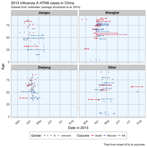
Gives this plot which shows that there are many missing values in the dates, so it is hard to draw a general conclusion.
Features
In Machine Learning-speak features are the variables used for model training. Using the right features dramatically influences the accuracy of the model.
Because we don’t have many features, I am keeping age as it is, but I am also generating new features:
- from the date information I am calculating the days between onset and outcome and between onset and hospitalisation
- I am converting gender into numeric values with 1 for female and 0 for male
- similarly, I am converting provinces to binary classifiers (yes == 1, no == 0) for Shanghai, Zhejiang, Jiangsu and other provinces
- the same binary classification is given for whether a case was hospitalised, and whether they had an early onset or early outcome (earlier than the median date)
# preparing the data frame for modeling
#
library(dplyr)

dataset <- fluH7N9.china.2013 %>%
  mutate(hospital = as.factor(ifelse(is.na(date.of.hospitalisation), 0, 1)),
         gender_f = as.factor(ifelse(gender == "f", 1, 0)),
         province_Jiangsu = as.factor(ifelse(province == "Jiangsu", 1, 0)),
         province_Shanghai = as.factor(ifelse(province == "Shanghai", 1, 0)),
         province_Zhejiang = as.factor(ifelse(province == "Zhejiang", 1, 0)),
         province_other = as.factor(ifelse(province == "Zhejiang" | province == "Jiangsu" | province == "Shanghai", 0, 1)),
         days_onset_to_outcome = as.numeric(as.character(gsub(" days", "",
                                      as.Date(as.character(date.of.outcome), format = "%Y-%m-%d") -
                                        as.Date(as.character(date.of.onset), format = "%Y-%m-%d")))),
         days_onset_to_hospital = as.numeric(as.character(gsub(" days", "",
                                      as.Date(as.character(date.of.hospitalisation), format = "%Y-%m-%d") -
                                        as.Date(as.character(date.of.onset), format = "%Y-%m-%d")))),
         age = as.numeric(as.character(age)),
         early_onset = as.factor(ifelse(date.of.onset < summary(fluH7N9.china.2013$date.of.onset)[[3]], 1, 0)),
         early_outcome = as.factor(ifelse(date.of.outcome < summary(fluH7N9.china.2013$date.of.outcome)[[3]], 1, 0))) %>%
  subset(select = -c(2:4, 6, 8))
rownames(dataset) <- dataset$case.ID
dataset <- dataset[, -1]Copy
Imputing missing values
When looking at the dataset I created for modeling, it is obvious that we have quite a few missing values. The missing values from the outcome column are what I want to predict but for the rest I would either have to remove the entire row from the data or impute the missing information. I decided to try the latter with the mice package.
# impute missing data
library(mice)
dataset_impute <- mice(dataset[, -1],  print = FALSE)

# recombine imputed data frame with the outcome column
dataset_complete <- merge(dataset[, 1, drop = FALSE], mice::complete(dataset_impute, 1), by = "row.names", all = TRUE)
rownames(dataset_complete) <- dataset_complete$Row.names
dataset_complete <- dataset_complete[, -1]
Copy
Test, train and validation datasets
For building the model, I am separating the imputed data frame into training and test data. Test data are the 57 cases with unknown outcome.
summary(dataset$outcome)
##   Death Recover    NA's
##      32      47      57Copy
The training data will be further devided for validation of the models: 70% of the training data will be kept for model building and the remaining 30% will be used for model testing. I am using the caret package for modeling.
train_index <- which(is.na(dataset_complete$outcome))
train_data <- dataset_complete[-train_index, ]
test_data  <- dataset_complete[train_index, -1]

library(caret)
set.seed(27)
val_index <- createDataPartition(train_data$outcome, p = 0.7, list=FALSE)
val_train_data <- train_data[val_index, ]
val_test_data  <- train_data[-val_index, ]
val_train_X <- val_train_data[,-1]
val_test_X <- val_test_data[,-1]Copy
Decision trees
To get an idea about how each feature contributes to the prediction of the outcome, I first built a decision tree based on the training data using rpart and rattle.
library(rpart)
library(rattle)
library(rpart.plot)
library(RColorBrewer)

set.seed(27)
fit <- rpart(outcome ~ .,
                    data = train_data,
                    method = "class",
                    control = rpart.control(xval = 10, minbucket = 2, cp = 0), parms = list(split = "information"))

fancyRpartPlot(fit)Copy
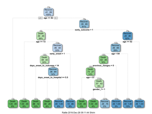
This randomly generated decision tree shows that cases with an early outcome were most likely to die when they were 68 or older, when they also had an early onset and when they were sick for fewer than 13 days. If a person was not among the first cases and was younger than 52, they had a good chance of recovering, but if they were 82 or older, they were more likely to die from the flu.
Feature Importance
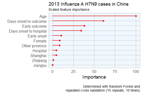
Not all of the features I created will be equally important to the model. The decision tree already gave me an idea of which features might be most important but I also want to estimate feature importance using a Random Forest approach with repeated cross validation.
# prepare training scheme
control <- trainControl(method = "repeatedcv", number = 10, repeats = 10)
# train the model
set.seed(27)
model <- train(outcome ~ ., data = train_data, method = "rf", preProcess = NULL, trControl = control)
# estimate variable importance
importance <- varImp(model, scale=TRUE)

# prepare for plotting
importance_df_1 <- importance$importance
importance_df_1$group <- rownames(importance_df_1)

importance_df_1$group <- mapvalues(importance_df_1$group,
                                           from = c("age", "hospital2", "gender_f2", "province_Jiangsu2", "province_Shanghai2", "province_Zhejiang2",
                                                    "province_other2", "days_onset_to_outcome", "days_onset_to_hospital", "early_onset2", "early_outcome2" ),
                                           to = c("Age", "Hospital", "Female", "Jiangsu", "Shanghai", "Zhejiang",
                                                    "Other province", "Days onset to outcome", "Days onset to hospital", "Early onset", "Early outcome" ))
f = importance_df_1[order(importance_df_1$Overall, decreasing = FALSE), "group"]

importance_df_2 <- importance_df_1
importance_df_2$Overall <- 0

importance_df <- rbind(importance_df_1, importance_df_2)

# setting factor levels
importance_df <- within(importance_df, group <- factor(group, levels = f))
importance_df_1 <- within(importance_df_1, group <- factor(group, levels = f))

ggplot() +
  geom_point(data = importance_df_1, aes(x = Overall, y = group, color = group), size = 2) +
  geom_path(data = importance_df, aes(x = Overall, y = group, color = group, group = group), size = 1) +
  scale_color_manual(values = rep(brewer.pal(1, "Set1")[1], 11)) +
  my_theme() +
  theme(legend.position = "none",
        axis.text.x = element_text(angle = 0, vjust = 0.5, hjust = 0.5)) +
  labs(
    x = "Importance",
    y = "",
    title = "2013 Influenza A H7N9 cases in China",
    subtitle = "Scaled feature importance",
    caption = "\nDetermined with Random Forest and
    repeated cross validation (10 repeats, 10 times)"
  )Copy
Feature Plot
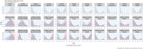
Before I start actually building models, I want to check whether the distribution of feature values is comparable between training, validation and test datasets.
# prepare for plotting
dataset_complete_gather <- dataset_complete %>%
  mutate(set = ifelse(rownames(dataset_complete) %in% rownames(test_data), "Test Data",
                               ifelse(rownames(dataset_complete) %in% rownames(val_train_data), "Validation Train Data",
                                      ifelse(rownames(dataset_complete) %in% rownames(val_test_data), "Validation Test Data", "NA"))),
         case_ID = rownames(.)) %>%
  gather(group, value, age:early_outcome)

dataset_complete_gather$group <- mapvalues(dataset_complete_gather$group,
                                           from = c("age", "hospital", "gender_f", "province_Jiangsu", "province_Shanghai", "province_Zhejiang",
                                                    "province_other", "days_onset_to_outcome", "days_onset_to_hospital", "early_onset", "early_outcome" ),
                                           to = c("Age", "Hospital", "Female", "Jiangsu", "Shanghai", "Zhejiang",
                                                    "Other province", "Days onset to outcome", "Days onset to hospital", "Early onset", "Early outcome" ))

ggplot(data = dataset_complete_gather, aes(x = as.numeric(value), fill = outcome, color = outcome)) +
  geom_density(alpha = 0.2) +
  geom_rug() +
  scale_color_brewer(palette="Set1", na.value = "grey50") +
  scale_fill_brewer(palette="Set1", na.value = "grey50") +
  my_theme() +
  facet_wrap(set ~ group, ncol = 11, scales = "free") +
  labs(
    x = "Value",
    y = "Density",
    title = "2013 Influenza A H7N9 cases in China",
    subtitle = "Features for classifying outcome",
    caption = "\nDensity distribution of all features used for classification of flu outcome."
  )
Copy
ggplot(subset(dataset_complete_gather, group == "Age" | group == "Days onset to hospital" | group == "Days onset to outcome"),
       aes(x=outcome, y=as.numeric(value), fill=set)) + geom_boxplot() +
  my_theme() +
  scale_fill_brewer(palette="Set1", type = "div ") +
  facet_wrap( ~ group, ncol = 3, scales = "free") +
  labs(
    fill = "",
    x = "Outcome",
    y = "Value",
    title = "2013 Influenza A H7N9 cases in China",
    subtitle = "Features for classifying outcome",
    caption = "\nBoxplot of the features age, days from onset to hospitalisation and days from onset to outcome."
  )Copy
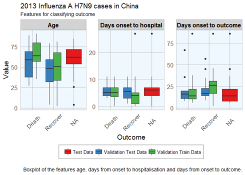
Gives this plot which luckily, the distributions looks reasonably similar between the validation and test data, except for a few outliers.
Comparing Machine Learning algorithms
Before I try to predict the outcome of the unknown cases, I am testing the models’ accuracy with the validation datasets on a couple of algorithms. I have chosen only a few more well known algorithms, but caret implements many more. I have chose to not do any preprocessing because I was worried that the different data distributions with continuous variables (e.g. age) and binary variables (i.e. 0, 1 classification of e.g. hospitalisation) would lead to problems.
Random Forest
Random Forests predictions are based on the generation of multiple classification trees. This model classified 14 out of 23 cases correctly.
set.seed(27)
model_rf <- caret::train(outcome ~ .,
                             data = val_train_data,
                             method = "rf",
                             preProcess = NULL,
                             trControl = trainControl(method = "repeatedcv", number = 10, repeats = 10, verboseIter = FALSE))

confusionMatrix(predict(model_rf, val_test_data[, -1]), val_test_data$outcome)
Copy
Elastic-Net Regularized Generalized Linear Models
Lasso or elastic net regularization for generalized linear model regression are based on linear regression models and is useful when we have feature correlation in our model. This model classified 13 out of 23 cases correctly.
set.seed(27)
model_glmnet <- caret::train(outcome ~ .,
                             data = val_train_data,
                             method = "glmnet",
                             preProcess = NULL,
                             trControl = trainControl(method = "repeatedcv", number = 10, repeats = 10, verboseIter = FALSE))
confusionMatrix(predict(model_glmnet, val_test_data[, -1]), val_test_data$outcome)
Copy
k-Nearest Neighbors
set.seed(27)
model_kknn <- caret::train(outcome ~ .,
                             data = val_train_data,
                             method = "kknn",
                             preProcess = NULL,
                             trControl = trainControl(method = "repeatedcv", number = 10, repeats = 10, verboseIter = FALSE))
confusionMatrix(predict(model_kknn, val_test_data[, -1]), val_test_data$outcome)Copy
Penalized Discriminant Analysis
set.seed(27)
model_pda <- caret::train(outcome ~ .,
                             data = val_train_data,
                             method = "pda",
                             preProcess = NULL,
                             trControl = trainControl(method = "repeatedcv", number = 10, repeats = 10, verboseIter = FALSE))
confusionMatrix(predict(model_pda, val_test_data[, -1]), val_test_data$outcome)Copy
Stabilized Linear Discriminant Analysis
Stabilized Linear Discriminant Analysis is designed for high-dimensional data and correlated co-variables. This model classified 15 out of 23 cases correctly.
set.seed(27)
model_slda <- caret::train(outcome ~ .,
                             data = val_train_data,
                             method = "slda",
                             preProcess = NULL,
                             trControl = trainControl(method = "repeatedcv", number = 10, repeats = 10, verboseIter = FALSE))
confusionMatrix(predict(model_slda, val_test_data[, -1]), val_test_data$outcome)Copy
Nearest Shrunken Centroids
Nearest Shrunken Centroids computes a standardized centroid for each class and shrinks each centroid toward the overall centroid for all classes. This model classified 15 out of 23 cases correctly.
set.seed(27)
model_pam <- caret::train(outcome ~ .,
                             data = val_train_data,
                             method = "pam",
                             preProcess = NULL,
                             trControl = trainControl(method = "repeatedcv", number = 10, repeats = 10, verboseIter = FALSE))
confusionMatrix(predict(model_pam, val_test_data[, -1]), val_test_data$outcome)Copy
Single C5.0 Tree
C5.0 is another tree-based modeling algorithm. This model classified 15 out of 23 cases correctly.
set.seed(27)
model_C5.0Tree <- caret::train(outcome ~ .,
                             data = val_train_data,
                             method = "C5.0Tree",
                             preProcess = NULL,
                             trControl = trainControl(method = "repeatedcv", number = 10, repeats = 10, verboseIter = FALSE))
confusionMatrix(predict(model_C5.0Tree, val_test_data[, -1]), val_test_data$outcome)Copy
Partial Least Squares
Partial least squares regression combined principal component analysis and multiple regression and is useful for modeling with correlated features. This model classified 15 out of 23 cases correctly.
set.seed(27)
model_pls <- caret::train(outcome ~ .,
                             data = val_train_data,
                             method = "pls",
                             preProcess = NULL,
                             trControl = trainControl(method = "repeatedcv", number = 10, repeats = 10, verboseIter = FALSE))
confusionMatrix(predict(model_pls, val_test_data[, -1]), val_test_data$outcome)Copy
Comparing accuracy of models
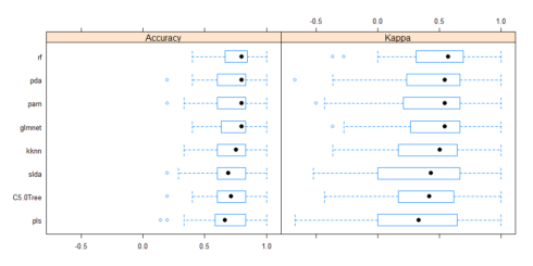
All models were similarly accurate.
# Create a list of models
models <- list(rf = model_rf, glmnet = model_glmnet, kknn = model_kknn, pda = model_pda, slda = model_slda,
               pam = model_pam, C5.0Tree = model_C5.0Tree, pls = model_pls)

# Resample the models
resample_results <- resamples(models)

# Generate a summary
summary(resample_results, metric = c("Kappa", "Accuracy"))
bwplot(resample_results , metric = c("Kappa","Accuracy"))Copy
Combined results of predicting validation test samples
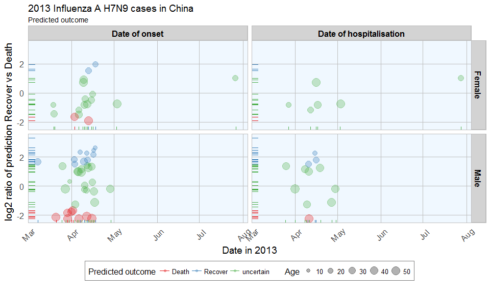
To compare the predictions from all models, I summed up the prediction probabilities for Death and Recovery from all models and calculated the log2 of the ratio between the summed probabilities for Recovery by the summed probabilities for Death. All cases with a log2 ratio bigger than 1.5 were defined as Recover, cases with a log2 ratio below -1.5 were defined as Death, and the remaining cases were defined as uncertain.
results <- data.frame(randomForest = predict(model_rf, newdata = val_test_data[, -1], type="prob"),
                      glmnet = predict(model_glmnet, newdata = val_test_data[, -1], type="prob"),
                      kknn = predict(model_kknn, newdata = val_test_data[, -1], type="prob"),
                      pda = predict(model_pda, newdata = val_test_data[, -1], type="prob"),
                      slda = predict(model_slda, newdata = val_test_data[, -1], type="prob"),
                      pam = predict(model_pam, newdata = val_test_data[, -1], type="prob"),
                      C5.0Tree = predict(model_C5.0Tree, newdata = val_test_data[, -1], type="prob"),
                      pls = predict(model_pls, newdata = val_test_data[, -1], type="prob"))

results$sum_Death <- rowSums(results[, grep("Death", colnames(results))])
results$sum_Recover <- rowSums(results[, grep("Recover", colnames(results))])
results$log2_ratio <- log2(results$sum_Recover/results$sum_Death)
results$true_outcome <- val_test_data$outcome
results$pred_outcome <- ifelse(results$log2_ratio > 1.5, "Recover", ifelse(results$log2_ratio < -1.5, "Death", "uncertain"))
results$prediction <- ifelse(results$pred_outcome == results$true_outcome, "CORRECT",
                             ifelse(results$pred_outcome == "uncertain", "uncertain", "wrong"))Copy
All predictions based on all models were either correct or uncertain.
Predicting unknown outcomes
The above models will now be used to predict the outcome of cases with unknown fate.
set.seed(27)
model_rf <- caret::train(outcome ~ .,
                             data = train_data,
                             method = "rf",
                             preProcess = NULL,
                             trControl = trainControl(method = "repeatedcv", number = 10, repeats = 10, verboseIter = FALSE))
model_glmnet <- caret::train(outcome ~ .,
                             data = train_data,
                             method = "glmnet",
                             preProcess = NULL,
                             trControl = trainControl(method = "repeatedcv", number = 10, repeats = 10, verboseIter = FALSE))
model_kknn <- caret::train(outcome ~ .,
                             data = train_data,
                             method = "kknn",
                             preProcess = NULL,
                             trControl = trainControl(method = "repeatedcv", number = 10, repeats = 10, verboseIter = FALSE))
model_pda <- caret::train(outcome ~ .,
                             data = train_data,
                             method = "pda",
                             preProcess = NULL,
                             trControl = trainControl(method = "repeatedcv", number = 10, repeats = 10, verboseIter = FALSE))
model_slda <- caret::train(outcome ~ .,
                             data = train_data,
                             method = "slda",
                             preProcess = NULL,
                             trControl = trainControl(method = "repeatedcv", number = 10, repeats = 10, verboseIter = FALSE))
model_pam <- caret::train(outcome ~ .,
                             data = train_data,
                             method = "pam",
                             preProcess = NULL,
                             trControl = trainControl(method = "repeatedcv", number = 10, repeats = 10, verboseIter = FALSE))
model_C5.0Tree <- caret::train(outcome ~ .,
                             data = train_data,
                             method = "C5.0Tree",
                             preProcess = NULL,
                             trControl = trainControl(method = "repeatedcv", number = 10, repeats = 10, verboseIter = FALSE))
model_pls <- caret::train(outcome ~ .,
                             data = train_data,
                             method = "pls",
                             preProcess = NULL,
                             trControl = trainControl(method = "repeatedcv", number = 10, repeats = 10, verboseIter = FALSE))

models <- list(rf = model_rf, glmnet = model_glmnet, kknn = model_kknn, pda = model_pda, slda = model_slda,
               pam = model_pam, C5.0Tree = model_C5.0Tree, pls = model_pls)

# Resample the models
resample_results <- resamples(models)

bwplot(resample_results , metric = c("Kappa","Accuracy"))Copy
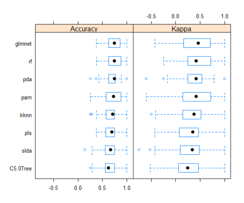
Here again, the accuracy is similar in all models. The final results are calculate as described above.
results <- data.frame(randomForest = predict(model_rf, newdata = test_data, type="prob"),
                      glmnet = predict(model_glmnet, newdata = test_data, type="prob"),
                      kknn = predict(model_kknn, newdata = test_data, type="prob"),
                      pda = predict(model_pda, newdata = test_data, type="prob"),
                      slda = predict(model_slda, newdata = test_data, type="prob"),
                      pam = predict(model_pam, newdata = test_data, type="prob"),
                      C5.0Tree = predict(model_C5.0Tree, newdata = test_data, type="prob"),
                      pls = predict(model_pls, newdata = test_data, type="prob"))

results$sum_Death <- rowSums(results[, grep("Death", colnames(results))])
results$sum_Recover <- rowSums(results[, grep("Recover", colnames(results))])
results$log2_ratio <- log2(results$sum_Recover/results$sum_Death)
results$predicted_outcome <- ifelse(results$log2_ratio > 1.5, "Recover", ifelse(results$log2_ratio < -1.5, "Death", "uncertain"))Copy
From 57 cases, 14 were defined as Recover, 10 as Death and 33 as uncertain.
results_combined <- merge(results[, -c(1:16)], fluH7N9.china.2013[which(fluH7N9.china.2013$case.ID %in% rownames(results)), ],
                          by.x = "row.names", by.y = "case.ID")
results_combined <- results_combined[, -c(2, 3, 8, 9)]
results_combined_gather <- results_combined %>%
  gather(group_dates, date, date.of.onset:date.of.hospitalisation)

results_combined_gather$group_dates <- factor(results_combined_gather$group_dates, levels = c("date.of.onset", "date.of.hospitalisation"))

results_combined_gather$group_dates <- mapvalues(results_combined_gather$group_dates, from = c("date.of.onset", "date.of.hospitalisation"),
                                             to = c("Date of onset", "Date of hospitalisation"))

results_combined_gather$gender <- mapvalues(results_combined_gather$gender, from = c("f", "m"),
                                             to = c("Female", "Male"))
levels(results_combined_gather$gender) <- c(levels(results_combined_gather$gender), "unknown")
results_combined_gather$gender[is.na(results_combined_gather$gender)] <- "unknown"
results_combined_gather$age <- as.numeric(as.character(results_combined_gather$age))

ggplot(data = results_combined_gather, aes(x = date, y = log2_ratio, color = predicted_outcome)) +
  geom_jitter(aes(size = age), alpha = 0.3) +
  geom_rug() +
  facet_grid(gender ~ group_dates) +
  labs(
    color = "Predicted outcome",
    size = "Age",
    x = "Date in 2013",
    y = "log2 ratio of prediction Recover vs Death",
    title = "2013 Influenza A H7N9 cases in China",
    subtitle = "Predicted outcome",
    caption = ""
  ) +
  my_theme() +
  scale_color_brewer(palette="Set1") +
  scale_fill_brewer(palette="Set1")Copy
The comparison of date of onset, data of hospitalisation, gender and age with predicted outcome shows that predicted deaths were associated with older age than predicted Recoveries. Date of onset does not show an obvious bias in either direction.
Conclusions
This dataset posed a couple of difficulties to begin with, like unequal distribution of data points across variables and missing data. This makes the modeling inherently prone to flaws. However, real life data isn’t perfect either, so I went ahead and tested the modeling success anyway. By accounting for uncertain classification with low predictions probability, the validation data could be classified accurately. However, for a more accurate model, these few cases don’t give enough information to reliably predict the outcome. More cases, more information (i.e. more features) and fewer missing data would improve the modeling outcome. Also, this example is only applicable for this specific case of flu. In order to be able to draw more general conclusions about flu outcome, other cases and additional information, for example on medical parameters like preexisting medical conditions, disase parameters, demographic information, etc. would be necessary. All in all, this dataset served as a nice example of the possibilities (and pitfalls) of machine learning applications and showcases a basic workflow for building prediction models with R.
If you have questions feel free to post a comment.
