Previously, I have published a blog post about how easy it is to train image classification models with Keras. What I did not show in that post was how to use the model for making predictions. This, I will do here.
But predictions alone are boring, so I'm adding explanations for the predictions using the lime package.
I have already written a few blog posts and gave talks:
- Looking beyond accuracy to improve trust in machine learning
- Explaining complex machine learning models with LIME
- Explaining Predictions of Machine Learning Models with LIME
- Explaining complex machine learning models with LIME
Neither of them applies LIME to image classification models, though. And with the new(ish) release from March of package by Thomas Lin Pedersen's, lime is now not only on CRAN but it natively supports Keras and image classification models.
Thomas wrote a very nice article about how to use keras and lime in R! Here, I am following this article to use Imagenet (VGG16) to make and explain predictions of fruit images and then I am extending the analysis to previous post and compare it with the pretrained net.
Loading libraries and models
library(keras)   # for working with neural nets
library(lime)    # for explaining models
library(magick)  # for preprocessing images
library(ggplot2) # for additional plotting
Loading the pretrained Imagenet model
model <- application_vgg16(weights = "imagenet", include_top = TRUE)
model
## Model
## ___________________________________________________________________________
## Layer (type)                     Output Shape                  Param #
## ===========================================================================
## input_1 (InputLayer)             (None, 224, 224, 3)           0
## ___________________________________________________________________________
## block1_conv1 (Conv2D)            (None, 224, 224, 64)          1792
## ___________________________________________________________________________
## block1_conv2 (Conv2D)            (None, 224, 224, 64)          36928
## ___________________________________________________________________________
## block1_pool (MaxPooling2D)       (None, 112, 112, 64)          0
## ___________________________________________________________________________
## block2_conv1 (Conv2D)            (None, 112, 112, 128)         73856
## ___________________________________________________________________________
## block2_conv2 (Conv2D)            (None, 112, 112, 128)         147584
## ___________________________________________________________________________
## block2_pool (MaxPooling2D)       (None, 56, 56, 128)           0
## ___________________________________________________________________________
## block3_conv1 (Conv2D)            (None, 56, 56, 256)           295168
## ___________________________________________________________________________
## block3_conv2 (Conv2D)            (None, 56, 56, 256)           590080
## ___________________________________________________________________________
## block3_conv3 (Conv2D)            (None, 56, 56, 256)           590080
## ___________________________________________________________________________
## block3_pool (MaxPooling2D)       (None, 28, 28, 256)           0
## ___________________________________________________________________________
## block4_conv1 (Conv2D)            (None, 28, 28, 512)           1180160
## ___________________________________________________________________________
## block4_conv2 (Conv2D)            (None, 28, 28, 512)           2359808
## ___________________________________________________________________________
## block4_conv3 (Conv2D)            (None, 28, 28, 512)           2359808
## ___________________________________________________________________________
## block4_pool (MaxPooling2D)       (None, 14, 14, 512)           0
## ___________________________________________________________________________
## block5_conv1 (Conv2D)            (None, 14, 14, 512)           2359808
## ___________________________________________________________________________
## block5_conv2 (Conv2D)            (None, 14, 14, 512)           2359808
## ___________________________________________________________________________
## block5_conv3 (Conv2D)            (None, 14, 14, 512)           2359808
## ___________________________________________________________________________
## block5_pool (MaxPooling2D)       (None, 7, 7, 512)             0
## ___________________________________________________________________________
## flatten (Flatten)                (None, 25088)                 0
## ___________________________________________________________________________
## fc1 (Dense)                      (None, 4096)                  102764544
## ___________________________________________________________________________
## fc2 (Dense)                      (None, 4096)                  16781312
## ___________________________________________________________________________
## predictions (Dense)              (None, 1000)                  4097000
## ===========================================================================
## Total params: 138,357,544
## Trainable params: 138,357,544
## Non-trainable params: 0
## ___________________________________________________________________________
Loading my own model from previous post
model2 <- load_model_hdf5(filepath = "/Users/shiringlander/Documents/Github/DL_AI/Tutti_Frutti/fruits-360/keras/fruits_checkpoints.h5")
model2
## Model
## ___________________________________________________________________________
## Layer (type)                     Output Shape                  Param #
## ===========================================================================
## conv2d_1 (Conv2D)                (None, 20, 20, 32)            896
## ___________________________________________________________________________
## activation_1 (Activation)        (None, 20, 20, 32)            0
## ___________________________________________________________________________
## conv2d_2 (Conv2D)                (None, 20, 20, 16)            4624
## ___________________________________________________________________________
## leaky_re_lu_1 (LeakyReLU)        (None, 20, 20, 16)            0
## ___________________________________________________________________________
## batch_normalization_1 (BatchNorm (None, 20, 20, 16)            64
## ___________________________________________________________________________
## max_pooling2d_1 (MaxPooling2D)   (None, 10, 10, 16)            0
## ___________________________________________________________________________
## dropout_1 (Dropout)              (None, 10, 10, 16)            0
## ___________________________________________________________________________
## flatten_1 (Flatten)              (None, 1600)                  0
## ___________________________________________________________________________
## dense_1 (Dense)                  (None, 100)                   160100
## ___________________________________________________________________________
## activation_2 (Activation)        (None, 100)                   0
## ___________________________________________________________________________
## dropout_2 (Dropout)              (None, 100)                   0
## ___________________________________________________________________________
## dense_2 (Dense)                  (None, 16)                    1616
## ___________________________________________________________________________
## activation_3 (Activation)        (None, 16)                    0
## ===========================================================================
## Total params: 167,300
## Trainable params: 167,268
## Non-trainable params: 32
## ___________________________________________________________________________
Load and prepare images
Here, I am loading and preprocessing two images of fruits (and yes, I am cheating a bit because I am choosing images where I expect my model to work as they are similar to the training images…).
Banana
test_image_files_path <- "/Users/shiringlander/Documents/Github/DL_AI/Tutti_Frutti/fruits-360/Test"
img <- image_read('https://upload.wikimedia.org/wikipedia/commons/thumb/8/8a/Banana-Single.jpg/272px-Banana-Single.jpg')
img_path <- file.path(test_image_files_path, "Banana", 'banana.jpg')
image_write(img, img_path)
#plot(as.raster(img))
Clementine
img2 <- image_read('https://cdn.pixabay.com/photo/2010/12/13/09/51/clementine-1792_1280.jpg')
img_path2 <- file.path(test_image_files_path, "Clementine", 'clementine.jpg')
image_write(img2, img_path2)
#plot(as.raster(img2))
Superpixels
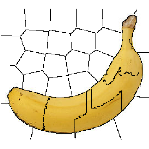
The segmentation of an image into superpixels are an important step in generating explanations for image models. It is both important that the segmentation is correct and follows meaningful patterns in the picture, but also that the size/number of superpixels are appropriate. If the important features in the image are chopped into too many segments the permutations will probably damage the picture beyond recognition in almost all cases leading to a poor or failing explanation model. As the size of the object of interest is varying it is impossible to set up hard rules for the number of superpixels to segment into – the larger the object is relative to the size of the image, the fewer superpixels should be generated. Using plot_superpixels it is possible to evaluate the superpixel parameters before starting the time-consuming explanation function. help(plot_superpixels)
plot_superpixels(img_path, n_superpixels = 35, weight = 10)
Gives this plot:
plot_superpixels(img_path2, n_superpixels = 50, weight = 20)
Gives this plot:

From the superpixel plots we can see that the clementine image has a higher resolution than the banana image.
Prepare images for Imagenet
image_prep <- function(x) {
  arrays <- lapply(x, function(path) {
    img <- image_load(path, target_size = c(224,224))
    x <- image_to_array(img)
    x <- array_reshape(x, c(1, dim(x)))
    x <- imagenet_preprocess_input(x)
  })
  do.call(abind::abind, c(arrays, list(along = 1)))
}
test predictions
res <- predict(model, image_prep(c(img_path, img_path2)))
imagenet_decode_predictions(res)
## [[1]]
## class_name class_description score
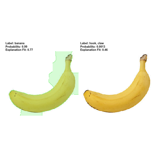
## 1 n07753592 banana 0.9929747581
## 2 n03532672 hook 0.0013420776
## 3 n07747607 orange 0.0010816186
## 4 n07749582 lemon 0.0010625814
## 5 n07716906 spaghetti_squash 0.0009176208
##
## [[2]]
## class_name class_description score
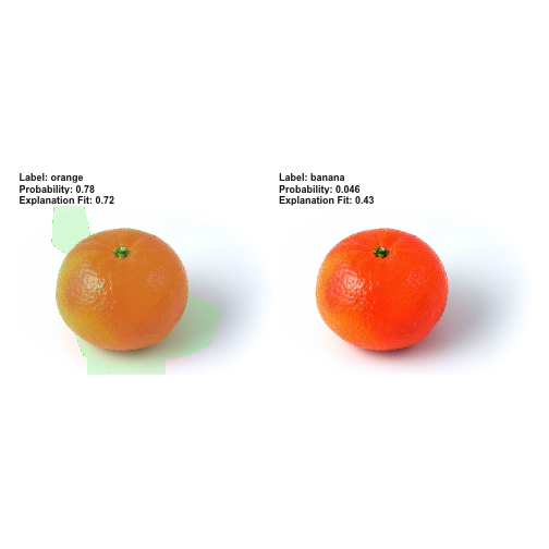
## 1 n07747607 orange 0.78233224
## 2 n07753592 banana 0.04653566
## 3 n07749582 lemon 0.03868873
## 4 n03134739 croquet_ball 0.03350329
## 5 n07745940 strawberry 0.01862431
load labels and train explainer
model_labels <- readRDS(system.file('extdata', 'imagenet_labels.rds', package = 'lime'))
explainer <- lime(c(img_path, img_path2), as_classifier(model, model_labels), image_prep)
Training the explainer explain() can take pretty long. It will be much faster with the smaller images in my own model but with the bigger Imagenet it takes a few minutes to run.
explanation <- explain(c(img_path, img_path2), explainer,
                       n_labels = 2, n_features = 35,
                       n_superpixels = 35, weight = 10,
                       background = "white")
plot_image_explanation() only supports showing one case at a time
plot_image_explanation(explanation)
Gives this plot:
clementine <- explanation[explanation$case == "clementine.jpg",]
plot_image_explanation(clementine)
Gives this plot:
Prepare images for my own model
Test predictions (analogous to training and validation images)
test_datagen <- image_data_generator(rescale = 1/255)
test_generator = flow_images_from_directory(
        test_image_files_path,
        test_datagen,
        target_size = c(20, 20),
        class_mode = 'categorical')
predictions <- as.data.frame(predict_generator(model2, test_generator, steps = 1))
load("/Users/shiringlander/Documents/Github/DL_AI/Tutti_Frutti/fruits-360/fruits_classes_indices.RData")
fruits_classes_indices_df <- data.frame(indices = unlist(fruits_classes_indices))
fruits_classes_indices_df <- fruits_classes_indices_df[order(fruits_classes_indices_df$indices), , drop = FALSE]
colnames(predictions) <- rownames(fruits_classes_indices_df)
t(round(predictions, digits = 2))
##             [,1] [,2]
## Kiwi           0    0
## Banana         0    1
## Apricot        0    0
## Avocado        0    0
## Cocos          0    0
## Clementine     1    0
## Mandarine      0    0
## Orange         0    0
## Limes          0    0
## Lemon          0    0
## Peach          0    0
## Plum           0    0
## Raspberry      0    0
## Strawberry     0    0
## Pineapple      0    0
## Pomegranate    0    0
for (i in 1:nrow(predictions)) {
  cat(i, ":")
  print(unlist(which.max(predictions[i, ])))
}
## 1 :Clementine
##          6
## 2 :Banana
##      2
This seems to be incompatible with lime, though (or if someone knows how it works, please let me know) – so I prepared the images similarly to the Imagenet images.
image_prep2 <- function(x) {
  arrays <- lapply(x, function(path) {
    img <- image_load(path, target_size = c(20, 20))
    x <- image_to_array(img)
    x <- reticulate::array_reshape(x, c(1, dim(x)))
    x <- x / 255
  })
  do.call(abind::abind, c(arrays, list(along = 1)))
}
prepare labels
fruits_classes_indices_l <- rownames(fruits_classes_indices_df)
names(fruits_classes_indices_l) <- unlist(fruits_classes_indices)
fruits_classes_indices_l
##             9            10             8             2            11
##        "Kiwi"      "Banana"     "Apricot"     "Avocado"       "Cocos"
##             3            13            14             7             6
##  "Clementine"   "Mandarine"      "Orange"       "Limes"       "Lemon"
##             1             5             0             4            15
##       "Peach"        "Plum"   "Raspberry"  "Strawberry"   "Pineapple"
##            12
## "Pomegranate"
train explainer
explainer2 <- lime(c(img_path, img_path2), as_classifier(model2, fruits_classes_indices_l), image_prep2)
explanation2 <- explain(c(img_path, img_path2), explainer2,
n_labels = 1, n_features = 20,
n_superpixels = 35, weight = 10,
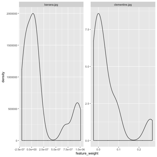
background = "white")plot feature weights to find a good threshold for plotting block (see below)
explanation2 %>%
  ggplot(aes(x = feature_weight)) +
    facet_wrap(~ case, scales = "free") +
    geom_density()
Gives this plot:
plot predictions
plot_image_explanation(explanation2, display = 'block', threshold = 5e-07)
Gives this plot:

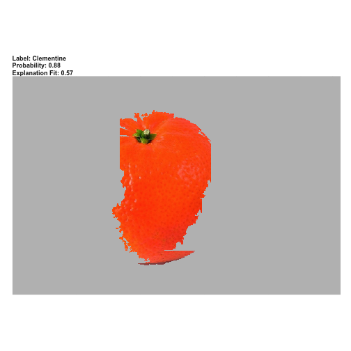
clementine2 <- explanation2[explanation2$case == "clementine.jpg",]
plot_image_explanation(clementine2, display = 'block', threshold = 0.16)
Gives this plot:
sessionInfo()
## R version 3.5.0 (2018-04-23)
## Platform: x86_64-apple-darwin15.6.0 (64-bit)
## Running under: macOS High Sierra 10.13.5
##
## Matrix products: default
## BLAS: /System/Library/Frameworks/Accelerate.framework/Versions/A/Frameworks/vecLib.framework/Versions/A/libBLAS.dylib
## LAPACK: /Library/Frameworks/R.framework/Versions/3.5/Resources/lib/libRlapack.dylib
##
## locale:
## [1] de_DE.UTF-8/de_DE.UTF-8/de_DE.UTF-8/C/de_DE.UTF-8/de_DE.UTF-8
##
## attached base packages:
## [1] stats     graphics  grDevices utils     datasets  methods   base
##
## other attached packages:
## [1] ggplot2_2.2.1    magick_1.9       lime_0.4.0       keras_2.1.6
## [5] knitr_1.20       RWordPress_0.2-3
##
## loaded via a namespace (and not attached):
##  [1] stringdist_0.9.5.1 reticulate_1.8     xfun_0.2
##  [4] reshape2_1.4.3     lattice_0.20-35    colorspace_1.3-2
##  [7] htmltools_0.3.6    yaml_2.1.19        base64enc_0.1-3
## [10] XML_3.98-1.11      rlang_0.2.1        pillar_1.2.3
## [13] later_0.7.3        foreach_1.4.4      plyr_1.8.4
## [16] tensorflow_1.8     stringr_1.3.1      munsell_0.5.0
## [19] blogdown_0.6       gtable_0.2.0       htmlwidgets_1.2
## [22] codetools_0.2-15   evaluate_0.10.1    labeling_0.3
## [25] httpuv_1.4.4.1     tfruns_1.3         curl_3.2
## [28] parallel_3.5.0     markdown_0.8       XMLRPC_0.3-0
## [31] highr_0.7          Rcpp_0.12.17       xtable_1.8-2
## [34] scales_0.5.0       backports_1.1.2    promises_1.0.1
## [37] jsonlite_1.5       abind_1.4-5        mime_0.5
## [40] digest_0.6.15      stringi_1.2.3      bookdown_0.7
## [43] shiny_1.1.0        grid_3.5.0         rprojroot_1.3-2
## [46] tools_3.5.0        bitops_1.0-6       magrittr_1.5
## [49] shinythemes_1.1.1  lazyeval_0.2.1     RCurl_1.95-4.10
## [52] glmnet_2.0-16      tibble_1.4.2       whisker_0.3-2
## [55] zeallot_0.1.0      Matrix_1.2-14      gower_0.1.2
## [58] assertthat_0.2.0   rmarkdown_1.10     iterators_1.0.9
## [61] R6_2.2.2           compiler_3.5.0