It could be the era of Deep Learning where it really doesn’t matter how big is your dataset or how many columns you’ve got. Still, a lot of Kaggle Competition Winners and Data Scientists emphasis on one thing that could put you on the top of the leaderboard in a Competition is “Feature Engineering”. Irrespective of how sophisticated your model is, good features will always help your Machine Learning Model building process better than others.
What is Feature engineering?
Features are nothing but columns/dimensions and Feature Engineering is the process of creating new Features or Predictors based on Domain Knowledge or Statistical Principles. Feature Engineering has always been around with Machine Learning but the latest in that is Automated Feature Engineering which has become a thing recently with Researchers started using Machine Learning itself to create new Features that can help in Model Accuracy. While most of the automated Featuring Engineering address numeric data, Text Data has always been left out in this race because of its inherent unstructured nature. No more, I could say.
textfeatures – R package
Michael Kearney, Assistant Professor in University of Missouri, well known in the R community for the modern twitter package rtweet, has come up with a new R packaged called textfeatures that basically generates a bunch of features for any text data that you supply. Before you dream of Deep Learning based Package for Automated Text Feature Engineering, This isn’t that. This uses very simple Text Analysis principles and generates features like Number of Upper Case letters, Number of Punctuations – plain simple stuff and nothing fancy but pretty useful ones.
Installation
textfeatures can be installed directly from CRAN and the development version is available on github.
install.packages("textfeatures")
Use Case
In this post, we will use textfeatures package to generate features for Fifa official world cup ios app reviews from the UK. We will R package itunesr to extract reviews and tidyverse for data manipulation and plotting.
Loading required Packages:
Let us load all the required packages.
#install.packages("itunesr")
#install.packages("textfeatures")
#install.packages("tidyverse")

library(itunesr)
library(textfeatures)
library(tidyverse)
Extracting recent Reviews:
#Get UK Reviews of Fifa official world cup ios app
#https://itunes.apple.com/us/app/2018-fifa-world-cup-russia/id756904853?mt=8

reviews1 <- getReviews(756904853,"GB",1)
reviews2 <- getReviews(756904853,"GB",2)
reviews3 <- getReviews(756904853,"GB",3)
reviews4 <- getReviews(756904853,"GB",4)

#Combining all the reviews into one dataframe
reviews <- rbind(reviews1,
                 reviews2,
                 reviews3,
                 reviews4)
textfeatures Magic Begins:
As we have got the reviews, Let us allow textfeatures to do its magic. We will use the function textfeatures() to do that.
#Combining all the reviews into one dataframe
reviews <- rbind(reviews1,
                 reviews2,
                 reviews3,
                 reviews4)

# generate text features
feat <- textfeatures(reviews$Review)

# check what all features generated
glimpse(feat)
Observations: 200
Variables: 17
$ n_chars         149, 13, 263, 189, 49, 338, 210, 186, 76, 14, 142, 114, 242, ...
$ n_commas        1, 0, 0, 0, 0, 1, 2, 1, 1, 0, 1, 1, 0, 3, 0, 0, 1, 0, 3, 1, 0...
$ n_digits        0, 0, 6, 3, 0, 4, 1, 0, 0, 0, 0, 0, 0, 3, 0, 0, 0, 3, 0, 0, 0...
$ n_exclaims      0, 0, 2, 2, 0, 0, 0, 1, 0, 0, 0, 0, 0, 0, 0, 0, 0, 1, 3, 0, 0...
$ n_extraspaces   1, 0, 0, 0, 0, 3, 0, 0, 1, 0, 0, 0, 1, 0, 0, 0, 0, 0, 0, 4, 0...
$ n_hashtags      0, 0, 0, 0, 0, 0, 0, 0, 0, 0, 0, 0, 0, 0, 0, 0, 0, 0, 0, 0, 0...
$ n_lowers        140, 11, 225, 170, 46, 323, 195, 178, 70, 12, 129, 106, 233, ...
$ n_lowersp       0.9400000, 0.8571429, 0.8560606, 0.9000000, 0.9400000, 0.9557...
$ n_mentions      0, 0, 0, 0, 0, 0, 0, 0, 0, 0, 0, 0, 0, 0, 0, 0, 0, 0, 0, 0, 0...
$ n_periods       2, 0, 5, 1, 0, 0, 3, 1, 2, 0, 2, 1, 1, 2, 0, 0, 4, 2, 0, 4, 0...
$ n_urls          0, 0, 0, 0, 0, 0, 0, 0, 0, 0, 0, 0, 0, 0, 0, 0, 0, 0, 0, 0, 0...
$ n_words         37, 2, 55, 45, 12, 80, 42, 41, 14, 3, 37, 28, 50, 16, 15, 8, ...
$ n_caps          4, 1, 12, 8, 2, 7, 3, 4, 2, 2, 6, 4, 6, 2, 3, 1, 6, 4, 29, 9,...
$ n_nonasciis     0, 0, 0, 0, 0, 0, 6, 0, 0, 0, 0, 0, 0, 0, 0, 0, 0, 0, 0, 0, 0...
$ n_puncts        2, 1, 7, 0, 1, 3, 4, 1, 1, 0, 4, 2, 2, 0, 1, 0, 1, 1, 0, 7, 2...
$ n_capsp         0.03333333, 0.14285714, 0.04924242, 0.04736842, 0.06000000, 0...
$ n_charsperword  3.947368, 4.666667, 4.714286, 4.130435, 3.846154, 4.185185, 4...
As you can see above, textfeatures have created 17 new features. Please note that these features will remain same for any text data.
Visualizing the outcome:
For this post, we wouldn’t build a Machine Learning Model but these features can very well be used for build a Classification model like Sentiment Classification or Category Classification.
But right now, we will just visualize the outcome with some features.
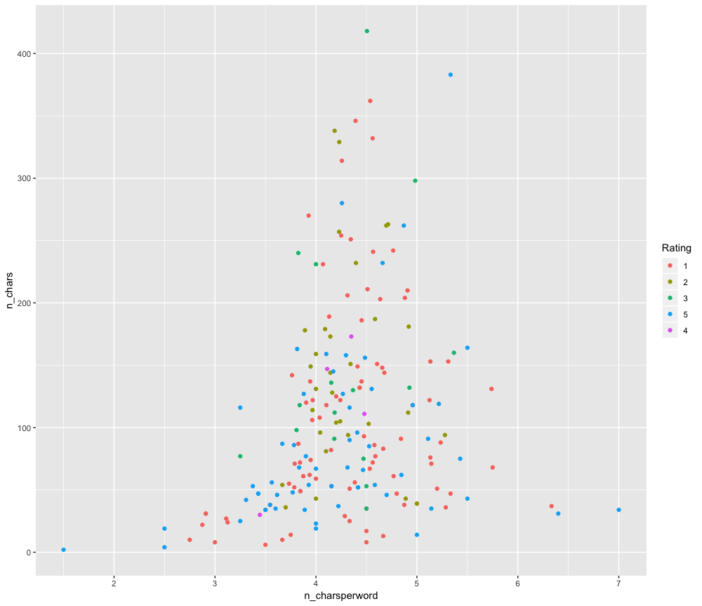
We can see if there’s any relations between a number of characters and number of characters per word, with respect to the Review rating. A hypothesis could be that people who give good rating wouldn’t write long or otherwise. We are not going to validate it here, but just visualizing using a scatter plot.
# merging features with original reviews
reviews_all %
  ggplot(aes(n_charsperword, n_chars, colour = Rating)) + geom_point()
Gives this plot:
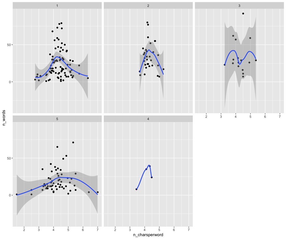
Let’s bring in a different perspective to the same hypothesis with a different plot but while comparing against a number of words instead of a number of characters.
reviews_all %>%
  ggplot(aes(n_charsperword, n_words)) + geom_point() +
  facet_wrap(~Rating) +
  stat_smooth()
Gives this plot:
Thus, you can use textfeatures to automatically generate new features and make a better understanding of your text data. Hope this post helps you get started with this beautiful package and if you’d like to know more on Text Analysis check out this tutorial by Julia Silge. The complete code used here is available on my github.
This is great. So, do we have any other feature engineering tool in R?
Nice post Abdul. Recommended plot: reviews_all %>% ggplot(aes(Rating, n_words, colour = Rating)) + geom_boxplot()
The people who writes less tend to rate 1 or 5!
https://uploads.disquscdn.com/images/19e07098433ab772cd2faefc790e6f1e59d8178a52b7b5380a36b00b469be4dc.png
That looks good 🙂 I think the base number would have an effect in this outcome.