In Data Science, As much as it is important to find patterns that repeat, It is also equally important to find anomalies that break those. This is actually very important in a place where we’ve got Time Series Data. Time Series Data is one where the data is spread across a Time Series Data.
Imagine, You run an online business like Amazon.com and you want to plan Server Resources for the next year – It is imperative that you need to know when your load is going to spike (or at least when did it spike in retrospective to believe it’ll repeat again) and that is where Time Series Anomaly Detection is what you are in need of. While there are some packages like Twitter’s AnomalyDetection that has been doing this job, there is a new candidate in the town – anomalize – that does something specific which no other Anomaly Detection packages were doing. That is Tidy Anomaly Detection.
Please note, The purpose of this article is to help you perform Anomaly Detection in R – The Tidy Way and not to teach you the principles and concepts of Anomaly Detection or Time Series Data.
What does Anomaly Detection in R – The Tidy Way mean?
Sorry to say this! Data Scientists who use R are known to write clumsy code – code that is not very readable and code that is not very efficient but this trend has been changing because of the tidy principle popularized by Hadley Wickham who supposedly doesn’t need any introduction in R universe, because his tidyverse is what contributes to the efficiency and work of a lot of R Data scientists. Now, this new package anomalize open-sourced by Business Science does Time Series Anomaly Detection that goes inline with other Tidyverse packages (or packages supporting tidy data) – with one of the most used Tidyverse functionality – compatibility with the pipe %>% operator to write readable and reproducible data pipeline.
anomalize – Installation
The Stable version of the R package anomalize is available on CRAN that could be installed like below:
install.packages('anomalize')
The latest development version of anomalize is available on github that could be installed like below:
#install.packages('devtools')
devtools::install_github("business-science/anomalize")
Considering that the development version doesn’t require compiling tools, It’s better to install the development version from github that would be more bug-free and with latest features.
Case – Bitcoin Price Anomaly Detection
It’s easier to learn a new concept or code piece by actually doing and relating it to what we are of. So, to understand the Tidy Anomaly Detection in R, We will try to detect anomalies in Bitcoin Price since 2017.
Loading Required Packages
We use the following 3 packages for to solve the above case:
library(anomalize) #tidy anomaly detectiom
library(tidyverse) #tidyverse packages like dplyr, ggplot, tidyr
library(coindeskr) #bitcoin price extraction from coindesk
Data Extraction
We use get_historic_price() from coindeskr to extract historic bitcoin price from Coindesk. The resulting dataframe is stored in the object btc
btc <- get_historic_price(start = "2017-01-01")
Data Preprocessing
For Anomaly Detection using anomalize, we need to have either a tibble or tibbletime object. Hence we have to convert the dataframe btc into a tibble object that follows a time series shape and store it in btc_ts.
btc_ts <- btc %>% rownames_to_column() %>% as.tibble() %>%
  mutate(date = as.Date(rowname)) %>% select(-one_of('rowname'))
Just looking at the head of btc_ts to see sample data:
head(btc_ts)
 Price date
1  998. 2017-01-01
2 1018. 2017-01-02
3 1031. 2017-01-03
4 1130. 2017-01-04
5 1006. 2017-01-05
6  896. 2017-01-06
Time Series Decomposition with Anomalies
One of the important things to do with Time Series data before starting with Time Series forecasting or Modelling is Time Series Decomposition where the Time series data is decomposed into Seasonal, Trend and remainder components. anomalize has got a function time_decompose() to perform the same. Once the components are decomposed, anomalize can detect and flag anomalies in the decomposed data of the reminder component which then could be visualized with plot_anomaly_decomposition() .
btc_ts %>%
  time_decompose(Price, method = "stl", frequency = "auto", trend = "auto") %>%
  anomalize(remainder, method = "gesd", alpha = 0.05, max_anoms = 0.2) %>%
  plot_anomaly_decomposition()
Gives this plot:
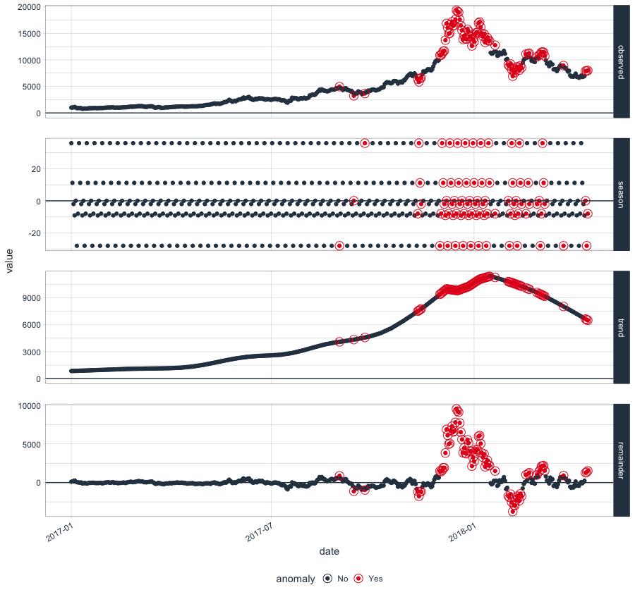
As you can see from the above code, the decomposition happens based on ‘stl’ method which is the common method of time series decomposition but if you have been using Twitter’s AnomalyDetection, then the same can be implemented in anomalize by combining time_decompose(method = “twitter”) with anomalize(method = "gesd"). Also the ‘stl’ method of decomposition can also be combined with anomalize(method = "iqr") for a different IQR based anomaly detection.
Anomaly Detection
Anomaly Detection and Plotting the detected anomalies are almost similar to what we saw above with Time Series Decomposition. It’s just that decomposed components after anomaly detection are recomposed back with time_recompose() and plotted with plot_anomalies() . The package itself automatically takes care of a lot of parameter setting like index, frequency and trend, making it easier to run anomaly detection out of the box with less prior expertise in the same domain.
btc_ts %>%
  time_decompose(Price) %>%
  anomalize(remainder) %>%
  time_recompose() %>%
  plot_anomalies(time_recomposed = TRUE, ncol = 3, alpha_dots = 0.5)
Gives this plot:
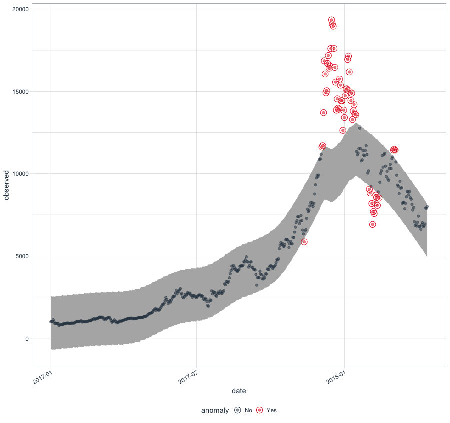
It could be very well inferred from the given plot how accurate the anomaly detection is finding out the Bitcoin Price madness that happened during the early 2018.
If you are interested in extracting the actual datapoints which are anomalies, the following code could be used:
btc_ts %>%
  time_decompose(Price) %>%
  anomalize(remainder) %>%
  time_recompose() %>%
  filter(anomaly == 'Yes')
Converting from tbl_df to tbl_time.
Auto-index message: index = date
frequency = 7 days
trend = 90.5 days
# A time tibble: 58 x 10
# Index: date
   date       observed   season trend remainder remainder_l1 remainder_l2 anomaly recomposed_l1

 1 2017-11-12    5857.  36.0    7599.    -1778.       -1551.        1672. Yes             6085.
 2 2017-12-04   11617.  11.2    9690.     1916.       -1551.        1672. Yes             8150.
 3 2017-12-05   11696.  -2.01   9790.     1908.       -1551.        1672. Yes             8237.
 4 2017-12-06   13709.  -9.11   9890.     3828.       -1551.        1672. Yes             8330.
 5 2017-12-07   16858.   0.0509 9990.     6868.       -1551.        1672. Yes             8439.
 6 2017-12-08   16057. -28.1    9971.     6114.       -1551.        1672. Yes             8393.
 7 2017-12-09   14913.  -8.03   9953.     4969.       -1551.        1672. Yes             8394.
 8 2017-12-10   15037.  36.0    9934.     5067.       -1551.        1672. Yes             8420.
 9 2017-12-11   16700.  11.2    9916.     6773.       -1551.        1672. Yes             8376.
10 2017-12-12   17178.  -2.01   9897.     7283.       -1551.        1672. Yes             8345.
# ... with 48 more rows, and 1 more variable: recomposed_l2
Thus, anomalize makes it easier to perform anomaly detection in R with cleaner code that also could be used in any data pipeline built using tidyverse. The code used here are available on my github. If you would like to know more about Time Series Forecasting in R, Check out Professor Rob Hyndman’s course on Datacamp.