This post aims to bring out some not-so-obvious subtle insights from analyzing TED Videos posted on TED.com. For those who do not know what is TED, Here’s the summary from Wikipedia: TED (Technology, Entertainment, Design) is a media organization which posts talks online for free distribution, under the slogan “ideas worth spreading”.
This analysis uses TED Talks dataset posted on Kaggle Datasets.
Data Description
Once the data is downloaded from the above link and unzipped, two files – 1. transcripts.csv, 2. ted_main.csv that are found to be read into R as below:
transcripts <- read.csv('../transcripts.csv',stringsAsFactors=F, header = T)
main <- read.csv('../ted_main.csv',stringsAsFactors=F, header = T)
ted_main.csv contains informations like Speaker Name, Talk Name, Event Name, Talk Duration, Comments, Video Views and much more for the videos made available on TED and transcripts.csv contains the entire talk transcript of the same talks.
Loading Libraries
library(dplyr); library(ggplot2); library(ggthemes);
Extract some basic info regarding the dataset.
nrow(main)
2550
2550 Video details are available in the main data frame. Since not all TED videos are extremely popular, let us see how many of those are with more than 1M views.
paste0('Total Number of videos with more than 1M views: ',main %>% filter(views > 1000000) %>% count() )
paste0('% of videos with more than 1M views: ', round((main %>% filter(views > 1000000) %>% count() / nrow(main))*100,2),'%')


'Total Number of videos with more than 1M views: 1503'
'% of videos with more than 1M views: 58.94%'
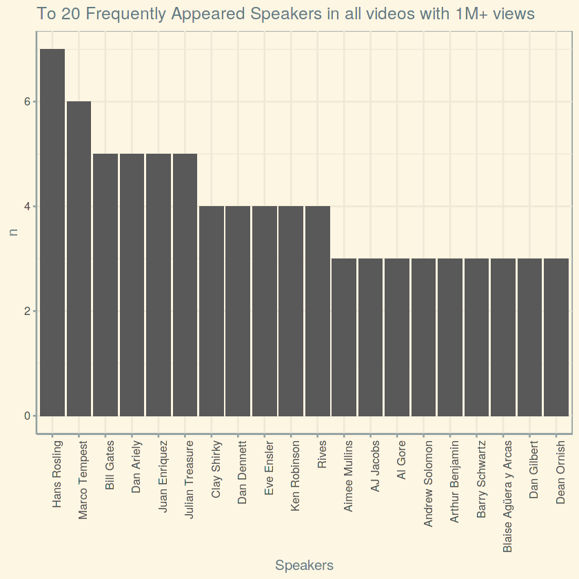
Being a one-trick-Pony is very easy in any business, so let us explore who are those among best of not-so-one-trick-ponies.
main %>% filter(views > 1000000) %>%
group_by(main_speaker) %>%
count() %>%
filter(n >2) %>%
arrange(desc(n)) %>%
head(20) %>%
ggplot() + geom_bar(aes(reorder(main_speaker,-n),n),stat='identity') + theme_solarized() +
theme(axis.text.x = element_text(angle = 90, hjust = 1)) + xlab('Speakers') +
ggtitle('To 20 Frequently Appeared Speakers in all videos with 1M+ views')
And the winner is none other than Mr. Hans Rosling whose Gapminder TED talk is always an inspiration for any Data Wiz.
Many a time, the amount of effort put gets translated to the effectiveness of the outcome, but the best is always getting things done with less effort – which in our case, more views with less time.
main %>% filter(views > 1000000) %>% arrange(duration) %>% slice(1:10) %>% select('name','duration','views','event')
name	duration	views	event
Derek Sivers: Weird, or just different?	162	2835976	TEDIndia 2009
Paolo Cardini: Forget multitasking, try monotasking	172	2324212	TEDGlobal 2012
Mitchell Joachim: Don't build your home, grow it!	176	1332785	TED2010
Arthur Benjamin: Teach statistics before calculus!	178	2175141	TED2009
Terry Moore: How to tie your shoes	179	6263759	TED2005
Malcolm London: "High School Training Ground"	180	1188177	TED Talks Education
Bobby McFerrin: Watch me play ... the audience!	184	3302312	World Science Festival
Derek Sivers: How to start a movement	189	6475731	TED2010
Bruno Maisonnier: Dance, tiny robots!	189	1193896	TEDxConcorde
Dean Ornish: Your genes are not your fate	192	1384333	TED2008
And the winner this time is, Derek Sivers, who happened to appear twice on the same list, donning two popular TED talks that are just under 6 minutes.
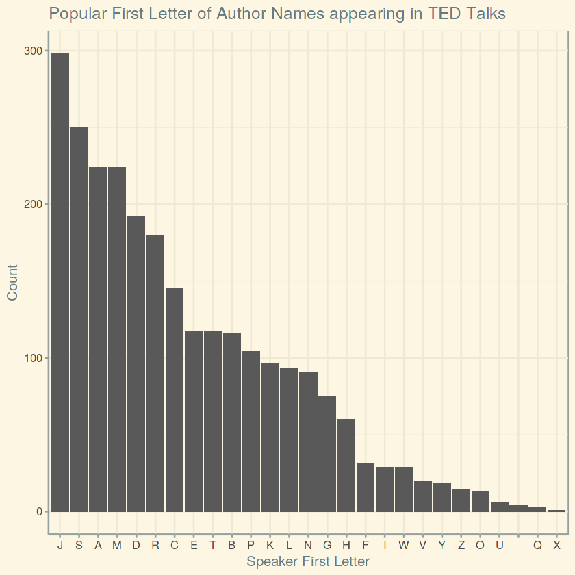
Malcolm Gladwell in his book Outliers presents an interesting case of how Date of Birth plays a role in Hockey team selection, so let us see if there is any magical first letter of the name that stands out among TED Speakers.
main$first_letter <- substr(main$main_speaker,1,1)
main %>%
group_by(first_letter = toupper(first_letter)) %>%
count() %>%
arrange(desc(n)) %>%
ggplot() +
geom_bar(aes(reorder(first_letter,-n),n),stat = 'identity') + theme_solarized() +
xlab('Speaker First Letter') +
ylab('Count') +
ggtitle('Popular First Letter of Author Names appearing in TED Talks')
And ‘J’ is the outstanding winner of the first-letter race that whose name holders frequently appeared on TED talks (Remember, correlation doesn’t mean causation!).
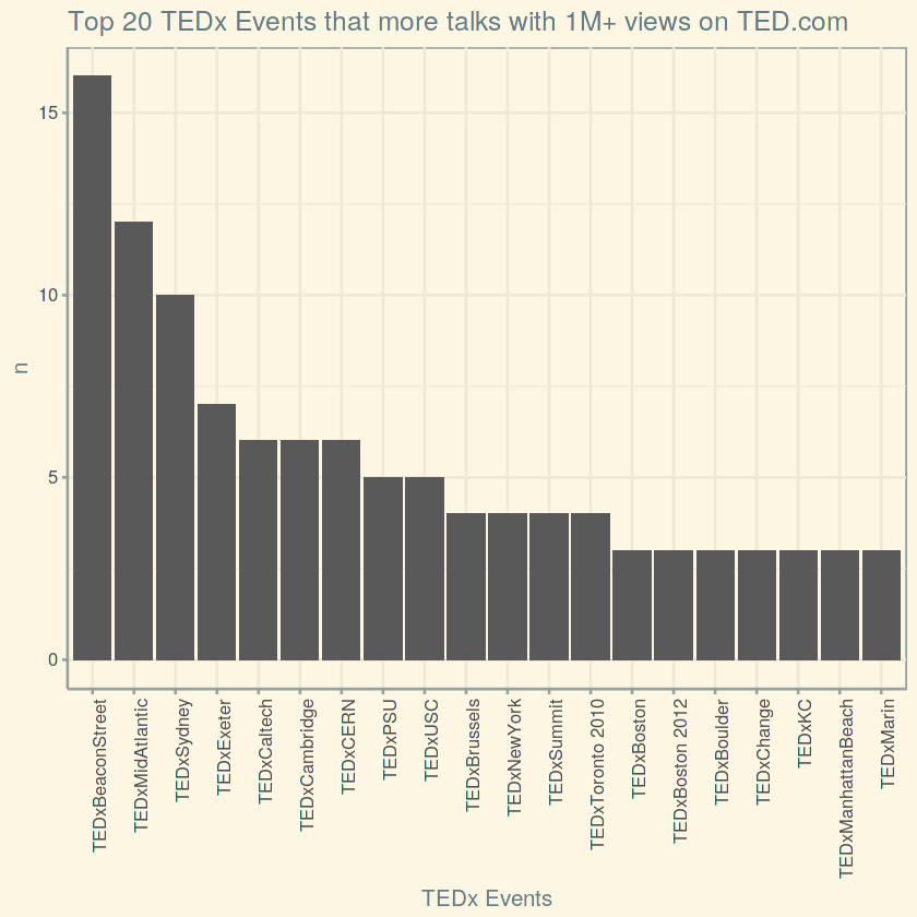
While TED primarily publishes videos from TED Global Event, some great TEDx videos get to feature on TED and let us analyze which TEDx chapter made it big.
tedx %>% filter(views > 1000000) %>%
group_by(event) %>%
count() %>%
filter(n >2) %>%
arrange(desc(n)) %>%
head(20) %>%
ggplot() + geom_bar(aes(reorder(event,-n),n),stat='identity') + theme_solarized() +
theme(axis.text.x = element_text(angle = 90, hjust = 1)) + xlab('TEDx Events') +
ggtitle('Top 20 TEDx Events that more talks with 1M+ views on TED.com')
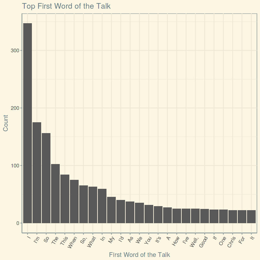
And Finally, let us analyze what is that magical (first) word that TED speakers usually start their talk with.
transcripts$first_word <- unlist(lapply(transcripts$transcript, function(x) strsplit(x," ")[[1]][1]))
transcripts %>% group_by(first_word) %>% count() %>% arrange(desc(n)) %>% head(25) %>%
ggplot() +
geom_bar(aes(reorder(first_word,-n),n),stat = 'identity') + theme_solarized() +
xlab('First Word of the Talk') +
ylab('Count') +
ggtitle('Top First Word of the Talk') +
theme(axis.text.x = element_text(angle = 60, hjust = 1))
And as most humans on the planet, most TED Speakers seem to start with ‘I’ (Narcissism, maybe?) and strangely Chris – the first name of Chris Anderson, the owner of TED appears on the same list too (Gratitude, maybe!).
This dataset still has a lot more interesting – subtle insights to be unveiled. The code used here is available on my Github.


