After months of collecting your data, after weeks of formatting it to the required format, after days of getting drown in the vast diversity of models available out there and choosing for a Bayesian approach, this is it, you fitted your model! Congrats, now the fun part of model checking comes into play.
About model checking
Taking a step back, models are a needed simplification of the reality. The world out there being too complex for interpretable models to capture every single interactions and data-generating mechanisms. Finding the right balance in model complexity to reliably answer the question at hand is the goal of any modelling exercice. There are several approaches that can help you in reaching that goal, the one presented in this post is based on gradual model expansion starting with a simple model and gradually expanding the model to include more structure or complexity where needed. In this approach model checking is key to identify where the model fails and how it can be improved.
More generally, model checking is a necessary step irrespective of the model complexity or the particular fitting approach. Even the most complex multilevel Bayesian models with spatio-temporal autocorrelation need checking so that reliable inference can be drawn. This post was greatly inspired by Michael Betancourt's Principled Bayesian Workflow, if you want to get more on model checking in a Bayesian context do head over there.
An example

Credit: Darkone / CC BY-SA (https://creativecommons.org/licenses/by-sa/2.0) URL
To guide us through this post we will use a relatively simple toy dataset. In this dataset we measured the plant height for 25 field scabious individuals (see the picture above) in 10 different plots together with soil nitrogen content. The aim being to explore the relation between soil nitrogen and field scabious plant height. So we will start with a simple model:
\[height_i \sim \mathcal{N}(\mu_i, \sigma)\]
\[\mu_i = \beta_0 + \beta_1 * nitrogen_i\]
Where i is the row index and \(\beta_0\), \(\beta_1\) and \(\sigma\) the model parameters to estimate.
This data can be loaded into your R environment:
# read the data
dat <- read.csv("https://raw.githubusercontent.com/lionel68/lionel68.github.io/master/_posts_data/knautia_height.csv")
Before we start: Package needed
To reproduce the R code in this post you will need the following packages:
- greta >= 0.3.1.9011, as of this post publication date this is the dev version that you can get by running:
devtools::install_github("greta-dev/greta")
greta uses the tensorflow python library to estimate the models, so you might encounter some issues with installation, do have a look at the dedicated website, also if you want to get more familiar with ways to fit greta models check this page. The concepts that will be covered here apply just as well to models fitted via JAGS or Stan or brms, so feel free to transpose this to your favorite model fitting engine.
- greta.checks, this package also need to be installed from github:
devtools::install_github("lionel68/greta.checks")
- bayesplot (from CRAN)
- DHARMa (from CRAN)
- coda (from CRAN)
- ggplot2 (from CRAN)
# load the libraries
library(greta)
library(greta.checks)
library(ggplot2)
Prior predictive checks
In Bayesian data analysis every model parameter require a prior which is a statistical distribution summarizing our knowledge prior to observing the data. Before fitting the model prior predictive checks allow checking that the model make sense with basic expectations.
Prior predictive checks function as follow:
- draw parameter values from the priors
- simulate multiple draws of the response based on the model
- summarize the response (i.e. take the mean)
In our toy example we could therefore check that the maximum value in the simulated new draws do not go beyond 2 meters, which are very unrealistic.
# define the priors
beta0 <- normal(0, 2)
beta1 <- normal(0, 1)
sd_res <- lognormal(0, 1)

# the linear predictor
# the mu in the model formula defined above
linpred <- beta0 + beta1 * dat$nitrogen

# turn the response into a greta array
height <- as_data(dat$height)

# the model
distribution(height) <- normal(linpred, sd_res)

# run prior checks
prior_check(height, fun = "max")
## [1] "80% of the 100 simulated response draws from the prior distributions had a max value between 0.86 and 10.66."
Across 100 simulated datasets based on the prior distribution, the maximum values in 80% of them was between 0.86 and 10.66cm.
Given our expert knowledge that it is not rare to see field scabious growing up to 1m, the priors should be a bit better tailored. An easy way to do it is to place a bit more information on the \(\beta_0\) and \(\beta_1\) parameter:
beta0 <- normal(50, 25)
beta1 <- normal(0, 5)

linpred <- beta0 + beta1 * dat$nitrogen

height <- as_data(dat$height)
distribution(height) <- normal(linpred, sd_res)

prior_check(height, fun = "max", probs = c(0.05, 0.95))
## [1] "90% of the 100 simulated response draws from the prior distributions had a max value between 22.17 and 96.23."
Better. With prior predictive distribution, we can check a lot of different aspect of the data and see if it correspond to our expectations. As the models grow more complex, prior checks are useful to check that the expected distribution is not going into areas that make little sense.
Checking convergence and sampling behavior
Once we are satisfied with our prior checks we can run a sampling algorithm to estimate the posterior distribution of the model parameters. This algorithm will basically travel through the parameter space for a certain number of steps (called iterations) following some rules. In Bayesian Data Analysis, the parameter distributions after sampling (the values of the parameters across all the iterations) is said to reliably estimate the posterior distributions once convergence is reached. Models can therefore only be interpreted after checking that convergence has been reached for all parameters.
Checking parameter convergence can be done graphically by looking at the trace plots of the parameters (caterpillar plots) or by using the Rhat metric, which should be 1.0 at convergence.
Let's do that on our toy example:
# define a model object
m <- model(beta0, beta1, sd_res)

# run a sampling algorithm
# with 100 iterations per chain for the warmup
m_fit <- mcmc(m, warmup = 100)
First we will visually check the trace plots:
bayesplot::mcmc_trace(m_fit)
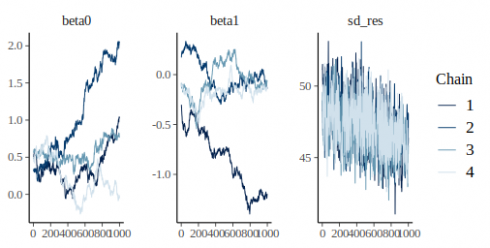
In this plot we have one panel per parameter, on the x axis are the 1000 iterations and on the y axis the parameter value. The different lines show the different chains.
Convergence can be visually assess from this type of graph by looking at two aspects:
- stationarity: the chains should not be moving up or down but rather be horizontally stable
- mixing: the chains should all be tightly intermixed
In our case convergence was very clearly not reached. An easy solution to that is to increase the number of warmup iterations, during warmup the sampler is tuning itself to the parameter and likelihood space, longer warmup means that the sampler will have more time to develop efficient rules to sample the posterior.
So we can try with 1000 warmup iterations:
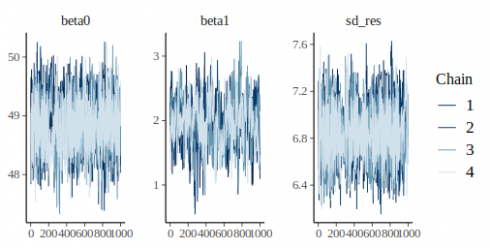
m_fit <- mcmc(m, warmup = 1000)
bayesplot::mcmc_trace(m_fit)
This looks much better, the chains are stationary and seem rather well-mixed. We can get numerical estimate of convegence using the Rhat metric:
coda::gelman.diag(m_fit)
## Potential scale reduction factors:
##
##        Point est. Upper C.I.
## beta0        1.00       1.00
## beta1        1.02       1.06
## sd_res       1.03       1.04
##
## Multivariate psrf
##
## 1.02
Rhat is 1 for all parameter, we can therefore reliably assume that the samples from the algorithm are a good representation of the posterior distribution. Traditionally a threshold of 1.1 is being used, parameters having Rhat below this value are said to be reliable, yet more recent work advocate for the use of stricter rules, i.e. 1.01 (see https://arxiv.org/pdf/1903.08008.pdf).
Posterior predictive checks
Using the posterior draws of the model parameters we can simulate new datasets and check if their distributions match the distribution of the original data.
This is in essence very similar to the prior predictive check, only that this time we use the posterior rather than the prior distribution of the model parameters.
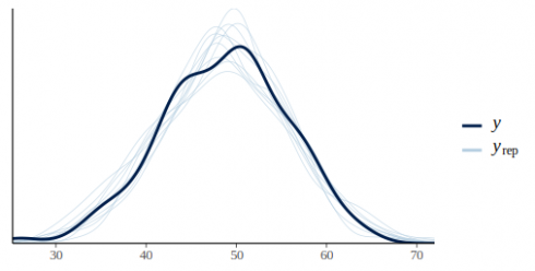
Let's put this in action by plotting the density from 50 simulates datasets against the original data:
pp_check(m_fit, height)
By default pp_check returns a density overlay of the posterior predictive distribution vs the original data.pp_check also convinently returns a ggplot2 object which can be further tailored if needed.
This graph looks pretty promising the light blue lines of the predictive posterior draws are more or less covering the dark line of the original data. In this model we ignored the effect of plots, we can check if this was ok by plotting the residuals against the plot id:
pp_check(m_fit, height, type = "error_scatter_avg_vs_x", x = dat$plot_id) +
  geom_hline(yintercept = 0, color = "red", size = 1.5) +
  scale_x_continuous(breaks = 1:10)
Using the fact that pp_check return a ggplot2 object we could easily add an horizontal line.
Now this graph show that some plots tend to have more positive residuals, while other more negative residuals. This is a cause of concern since normally the residuals should be uniformly distributed. We can check this by also plotting the observed average per plot against the posterior predictions:
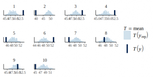
pp_check(m_fit, height, type = "stat_grouped", group = dat$plot_id, stat = "mean", nsim = 300)
The model assume no effect of the plot on the observations but from this graph it is clear that some plot such as plot 2 or 10 have lower average than others.
So let's expand our model by allowing the plots to have different average values:
beta0 <- normal(50, 5)
beta1 <- normal(0, 5)
# parameter for the deviation
# in the plot average
sd_plot <- lognormal(0, 1)
# plot-level deviation from overall average
plot_eff <- normal(0, sd_plot, dim = max(dat$plot_id))

# linear predictor for the mean
linpred <- beta0 + beta1 * dat$nitrogen + plot_eff[dat$plot_id]

# residual deviation
sd_res <- lognormal(0, 1)

height <- as_data(dat$height)
distribution(height) <- normal(linpred, sd_res)
This model allow plot average to deviate from the overall average. We can do our prior checks:
prior_check(height, fun = "mean")
## [1] "80% of the 100 simulated response draws from the prior distributions had a mean value between 43.17 and 56.04."
Looks plausible, let's fit the model and directly get the rhat:
m_var <- model(beta0, beta1, sd_plot, sd_res)
# to make the sampling algorithm more efficient
# we increase the number of leapfrog steps
m_var_fit <- mcmc(m_var, hmc(Lmin = 35, Lmax = 50))
coda::gelman.diag(m_var_fit)
## Potential scale reduction factors:
##
##         Point est. Upper C.I.
## beta0         1.04       1.09
## beta1         1.00       1.00
## sd_plot       1.00       1.01
## sd_res        1.00       1.00
##
## Multivariate psrf
##
## 1.13
Could be better but we’ll continue and check our posterior predictive plots:
pp_check(m_var_fit, height, type = "stat_grouped", group = dat$plot_id, stat = "mean", nsim = 300)
Much better, the model seems to have captured this source of variation, and we can look back at the residual plot:
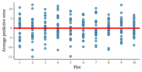
pp_check(m_var_fit, height, type = "error_scatter_avg_vs_x", nsim = 100, x = dat$plot_id) +
  geom_hline(yintercept = 0, color = "red", size = 1.5) +
  scale_x_continuous(breaks = 1:10) +
  labs(x= "Plot")
This graph also looks ok now, the residuals are evenly spread above and below the red line for all plots.
Specific themes: spatial autocorrelation and more
Another very useful package to check your model is the DHARMa package, it provides a lot of function to check other model pathologies such as under or overdispersion, spatial autocorrelation and much more.
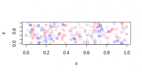
The plants that we measured are more or less close together, the lng and lat columns in the dataset are the spatial coordinates of the individuals. So we could ask ourselves: are plants closer together more likely to share similar values, in other words, are there some indications of spatial autocorrelations?
Let's check it:
sims <- simulate_residual(m_var_fit, height, linpred, nsim = 100)
The function simulate_residual returns a DHARMa object that opens up the vast function treasure of that package, we can test for spatial autocorrelation:
DHARMa::testSpatialAutocorrelation(sims, x = dat$lng, y = dat$lat)##
##  DHARMa Moran's I test for spatial autocorrelation
##
## data:  sims
## observed = 0.0104763, expected = -0.0040161, sd = 0.0074389, p-value =
## 0.05139
## alternative hypothesis: Spatial autocorrelation
There are little indication for spatial autocorrelation to be present in our model.
Conclusion
In this post we saw what are the standard model checks for Bayesian data analysis (convergence + posterior predictive checks), running these checks is very straightforward thanks to different R packages.
Building and fitting complex models is every day easier, yet sometime these complex models act a bit like a black box to the data analyst. In that sense following a gradual model expansion approach provide some advantages, starting simple, discovering where the model fails and expanding where needed.
All of this is easier said than done but it is my hope that this post gave you some helpful hints on how to check Bayesian models and gain both understanding and confidence in them. Any feedbacks, comments or criticisms, do reach out!
Happy checking!
