In the latest issue of the British Medical Journal (BMJ), I read a paper by Budhathoki et al. that investigated the association between vitamin D (serum 25-hydroxyvitamin D) and cancer in the Japenese population. The authors reported that high levels of vitamin D were associated with low risk of cancer. There is a large evidence base supporting the beneficial role of vitamin D in lowering the risk of chronic diseases and mortality. Therefore, I got motivated to explore the levels of Vitamin D in the U.S. using the data from National Health and Nutrition Examination Survey (NHANES).
This analysis is composed of three parts. First, I will calculate the prevalence of vitamin D status (i.e., deficiency, inadequacy, and sufficiency) in the United States for 2009-2010 and will build bar plots. Second, I will conduct a stratified analysis by gender, race, and pregnancy status to visualize proportions of inadequacy and deficiency. In the end, to establish the trends of vitamin D, I will build the trajectories from 2001 to 2010. To account for variability of vitamin D levels by age and season, the prevalences of deficiency and inadequacy will be calculated in using multivariable logistic regression.
Libraries and Datasets
Load the neccessary libraries
library(tidyverse)
library(RNHANES)
library(ggsci)
library(ggthemes)
Upload NHANES data from 2001 to 2010 and select the variables of interest.
d01 = nhanes_load_data("VID_B", "2001-2002") %>%
  transmute(SEQN=SEQN, vitD=LBDVIDMS, wave=cycle) %>%
  select(SEQN, vitD, wave) %>%
  left_join(nhanes_load_data("DEMO_B", "2001-2002"), by="SEQN") %>%
  select(SEQN, vitD, wave, RIAGENDR, RIDAGEYR, RIDEXPRG, RIDRETH1, WTMEC2YR, RIDEXMON)

d03 = nhanes_load_data("VID_C", "2003-2004") %>%
  transmute(SEQN=SEQN, vitD=LBDVIDMS, wave=cycle) %>%
  select(SEQN, vitD, wave) %>%
  left_join(nhanes_load_data("DEMO_C", "2003-2004"), by="SEQN") %>%
  select(SEQN, vitD, wave, RIAGENDR, RIDAGEYR,RIDRETH1, WTMEC2YR, RIDEXMON, RIDEXPRG)

d05 = nhanes_load_data("VID_D", "2005-2006") %>%
  transmute(SEQN=SEQN, vitD=LBDVIDMS, wave=cycle) %>%
  select(SEQN, vitD, wave) %>%
  left_join(nhanes_load_data("DEMO_D", "2005-2006"), by="SEQN") %>%
  select(SEQN, vitD, wave, RIAGENDR, RIDAGEYR, RIDRETH1, WTMEC2YR, RIDEXMON, RIDEXPRG)

d07 = nhanes_load_data("VID_E", "2007-2008") %>%
  transmute(SEQN=SEQN, vitD=LBXVIDMS, wave=cycle) %>%
  select(SEQN, vitD, wave) %>%
  left_join(nhanes_load_data("DEMO_E", "2007-2008"), by="SEQN") %>%
  select(SEQN, vitD, wave, RIAGENDR, RIDAGEYR, RIDRETH1, WTMEC2YR, RIDEXMON, RIDEXPRG)

d09 = nhanes_load_data("VID_F", "2009-2010") %>%
  transmute(SEQN=SEQN, vitD=LBXVIDMS, wave=cycle) %>%
  select(SEQN, vitD, wave) %>%
  left_join(nhanes_load_data("DEMO_F", "2009-2010"), by="SEQN") %>%
  select(SEQN, vitD, wave, RIAGENDR,RIDAGEYR, RIDRETH1, WTMEC2YR, RIDEXMON, RIDEXPRG)
The datasets includes following variables:
-
* SEQN: id
* RIAGENDR: gender
* RIDAGEYR: age in years
* RIDRETH1: race/origin
* vitD: vitaminD (nmol/L)
* wave: cycle of survey
* WTMEC2YR: 2-year sample weights
* RIDEXPRG: pregnancy status
* RIDEXMON: season (six month time period)
Data Cleaning
I will combine all dataset with using the function rbind as all columns of each dataset have same variable names.
all = rbind(d01, d03, d05, d07, d09)
Next, I will exclude participants with no information on vitamin D or with vitamin D larger than 125 nm/L (1% of the sample). Vitamin D > 125 nmol/l is considered to have possibly harmful effects and it is not the purpose of the current analysis. Also, I will group vitamin D levels according to Institute of Medicine guidelines, and I will recode gender and race.
Institute of Medicine cutoffs for Vitamin D
-
* Vitamin D deficiency: Serum 25OHD less than 30 nmol/L (12 ng/mL)
* Vitamin D inadequacy: Serum 25OHD 30-49 nmol/L (12-19 ng/mL)
* Vitamin D sufficiency: Serum 25OHD 50-125 nmol/L (20-50 ng/mL)
clean_all = all %>%
  filter(!is.na(vitD), vitD < 125) %>%
  mutate(
    gender = recode_factor(RIAGENDR,
                           `1` = "Males",
                           `2` = "Females"),
     race = recode_factor(RIDRETH1,
                         `1` = "Mexian American",
                         `2` = "Hispanic",
                         `3` = "Non-Hispanic, White",
                         `4` = "Non-Hispanic, Black",
                         `5` = "Others"),
   vitD_group = case_when(
      vitD < 30 ~ "Deficiency",
      vitD >= 30 & vitD < 50 ~ "Inadequacy",
      vitD >= 50 & vitD <= 125 ~ "Sufficiency"),
   pregnancy = if_else(RIDEXPRG == 1, "Yes", "No", "No")) %>%
  select(-RIDEXPRG)
Vitamine D status in NHANES 2009-2010
I will plot the status of vitamin D in 2009-2010 survey. The 2009-2010 survey is the latest survey where levels of vitamin D were measured.
clean_all %>%
  filter(wave == "2009-2010") %>%
  group_by(vitD_group) %>%
  summarise(n = n()) %>%
  mutate("%" = round(n/sum(n), 3) *100) %>%
  ggplot(., aes(x=vitD_group, y=`%`)) +
  geom_bar(stat = "identity", width = 0.5, fill = "#B24745") +
  geom_text(aes(label = paste0(`%`, "%"), y = `%`),
            vjust = 1.5, size = 3, color = "#FFFFFF") +
  theme_hc() +
  theme(text = element_text(family = "serif", size = 11), legend.position="none") +
  labs(
    title = "Vitamin D status in the United States: NHANES 2009-2010",
    subtitle = "",
    caption = "",
    x = "Vitamin D Status",
    y = "Percentage, %"
    )
This gives the plot:
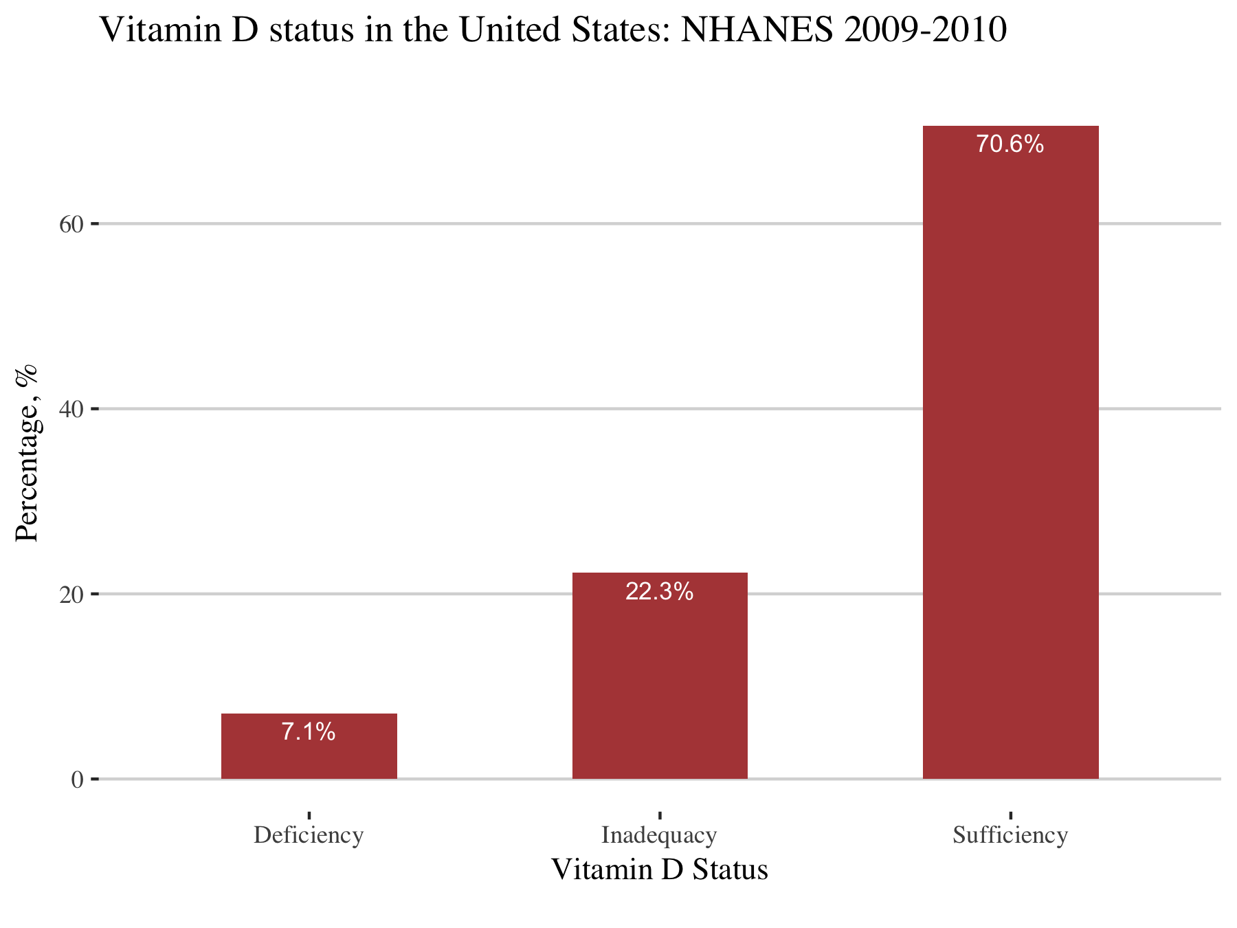
As it is shown above two-thirds (70.6%) of the population had sufficient levels of vitamin D, while 22.3% have inadequacy and 7.1% have a deficiency in vitamin D.
Age and season adjusted prevalences of Vitamin D status in USA, 2001 – 2010
Given that levels of vitamin D are sensible to season and age, I will take them into account. During the winter the levels of Vitamin D are lower as the skin is not exposed to the sun, while in summer levels of Vitamine D increases. Age has a similar importance as levels of Vitamin D drops in older individuals. Therefore, the prevalences of vitamin D will be age- and season-adjusted.
In order to calculate the adjusted age and season values of vitamin D I will fit a logistic regression analysis and will use the function predict to obtain the predicted (adjusted) proportions of vitamin D for each individual. First, I will create a dummy variable for inadequacy and deficiency of vitamin D as in logisitic regression the dependent variable should be coded 0 or 1.
reg_dt = clean_all %>%
  mutate(
    vitD_inad = if_else(vitD_group == "Inadequacy", 1, 0),
    vitD_defi = if_else(vitD_group == "Deficiency", 1, 0)
  )
Now we have two new variables vitD_inad and vitD_defi for inadequacy and deficiency, respectively. Let’s fit the logistic regression adjusted by age and season and stratified by gender and survey.
Logistic regression in males:
m2001 = reg_dt %>%
  filter(wave == "2001-2002", gender == "Males")
m2003 = reg_dt %>%
  filter(wave == "2003-2004", gender == "Males")
m2005 = reg_dt %>%
  filter(wave == "2005-2006", gender == "Males")
m2007 = reg_dt %>%
  filter(wave == "2007-2008", gender == "Males")
m2009 = reg_dt %>%
  filter(wave == "2009-2010", gender == "Males")

# Inadequancy
adj_vitD_inad = predict(
  glm(vitD_inad ~ RIDAGEYR + RIDEXMON, family=binomial, data = m2001),
  type="response")
adj2001_inad = cbind(m2001, adj_vitD_inad)
adj_vitD_inad = predict(
  glm(vitD_inad ~ RIDAGEYR + RIDEXMON, family=binomial, data = m2003),
  type="response")
adj2003_inad = cbind(m2003, adj_vitD_inad)
adj_vitD_inad = predict(
  glm(vitD_inad ~ RIDAGEYR + RIDEXMON, family=binomial, data = m2005),
  type="response")
adj2005_inad = cbind(m2005, adj_vitD_inad)
adj_vitD_inad = predict(
  glm(vitD_inad ~ RIDAGEYR + RIDEXMON, family=binomial, data = m2007),
  type="response")
adj2007_inad = cbind(m2007, adj_vitD_inad)
adj_vitD_inad = predict(
  glm(vitD_inad ~ RIDAGEYR + RIDEXMON, family=binomial, data = m2009),
  type="response")
adj2009_inad = cbind(m2009, adj_vitD_inad)

male_dat_inad = bind_rows(adj2001_inad, adj2003_inad, adj2005_inad, adj2007_inad, adj2009_inad) %>%
  select(SEQN, adj_vitD_inad)

# Deficiency
adj_vitD_defi = predict(
  glm(vitD_defi ~ RIDAGEYR + RIDEXMON, family=binomial, data = m2001),
  type="response")
adj2001_defi = cbind(m2001, adj_vitD_defi)
adj_vitD_defi = predict(
  glm(vitD_defi ~ RIDAGEYR + RIDEXMON, family=binomial, data = m2003),
  type="response")
adj2003_defi = cbind(m2003, adj_vitD_defi)
adj_vitD_defi = predict(
  glm(vitD_defi ~ RIDAGEYR + RIDEXMON, family=binomial, data = m2005),
  type="response")
adj2005_defi = cbind(m2005, adj_vitD_defi)
adj_vitD_defi = predict(
  glm(vitD_defi ~ RIDAGEYR + RIDEXMON, family=binomial, data = m2007),
  type="response")
adj2007_defi = cbind(m2007, adj_vitD_defi)
adj_vitD_defi = predict(
  glm(vitD_defi ~ RIDAGEYR + RIDEXMON, family=binomial, data = m2009),
  type="response")
adj2009_defi = cbind(m2009, adj_vitD_defi)

male_dat_defi = bind_rows(adj2001_defi, adj2003_defi, adj2005_defi, adj2007_defi, adj2009_defi) %>%
  select(SEQN, adj_vitD_defi)
Logistic regression in females:
m2001 = reg_dt %>%
  filter(wave == "2001-2002", gender == "Females")
m2003 = reg_dt %>%
  filter(wave == "2003-2004", gender == "Females")
m2005 = reg_dt %>%
  filter(wave == "2005-2006", gender == "Females")
m2007 = reg_dt %>%
  filter(wave == "2007-2008", gender == "Females")
m2009 = reg_dt %>%
  filter(wave == "2009-2010", gender == "Females")

# Inadequancy
adj_vitD_inad = predict(
  glm(vitD_inad ~ RIDAGEYR + RIDEXMON, family=binomial, data = m2001),
  type="response")
adj2001_inad = cbind(m2001, adj_vitD_inad)
adj_vitD_inad = predict(glm(
  vitD_inad ~ RIDAGEYR + RIDEXMON, family=binomial, data = m2003),
  type="response")
adj2003_inad = cbind(m2003, adj_vitD_inad)
adj_vitD_inad = predict(glm(
  vitD_inad ~ RIDAGEYR + RIDEXMON, family=binomial, data = m2005),
  type="response")
adj2005_inad = cbind(m2005, adj_vitD_inad)
adj_vitD_inad = predict(glm(
  vitD_inad ~ RIDAGEYR + RIDEXMON, family=binomial, data = m2007),
  type="response")
adj2007_inad = cbind(m2007, adj_vitD_inad)
adj_vitD_inad = predict(
  glm(vitD_inad ~ RIDAGEYR + RIDEXMON, family=binomial, data = m2009),
  type="response")
adj2009_inad = cbind(m2009, adj_vitD_inad)
female_dat_inad = bind_rows(adj2001_inad, adj2003_inad, adj2005_inad, adj2007_inad, adj2009_inad) %>%
  select(SEQN, adj_vitD_inad)

# Deficiency
adj_vitD_defi = predict(
  glm(vitD_defi ~ RIDAGEYR + RIDEXMON, family=binomial, data = m2001),
  type="response")
adj2001_defi = cbind(m2001, adj_vitD_defi)
adj_vitD_defi = predict(
  glm(vitD_defi ~ RIDAGEYR + RIDEXMON, family=binomial, data = m2003),
  type="response")
adj2003_defi = cbind(m2003, adj_vitD_defi)
adj_vitD_defi = predict(
  glm(vitD_defi ~ RIDAGEYR + RIDEXMON, family=binomial, data = m2005),
  type="response")
adj2005_defi = cbind(m2005, adj_vitD_defi)
adj_vitD_defi = predict(
  glm(vitD_defi ~ RIDAGEYR + RIDEXMON, family=binomial, data = m2007),
  type="response")
adj2007_defi = cbind(m2007, adj_vitD_defi)
adj_vitD_defi = predict(glm(
  vitD_defi ~ RIDAGEYR + RIDEXMON, family=binomial, data = m2009),
  type="response")
adj2009_defi = cbind(m2009, adj_vitD_defi)
female_dat_defi = bind_rows(adj2001_defi, adj2003_defi, adj2005_defi, adj2007_defi, adj2009_defi) %>%
  select(SEQN, adj_vitD_defi)
Merge males and females together
reg_dat01 = rbind(male_dat_inad, female_dat_inad)
reg_dat02 = rbind(male_dat_defi, female_dat_defi)
reg_dat = left_join(reg_dt, reg_dat01) %>%
  left_join(reg_dat02) %>%
  mutate(
    adj_vitD_inad = round(adj_vitD_inad*100, 1),
    adj_vitD_defi = round(adj_vitD_defi*100, 1)
  )
In the dataset reg_dat I have two new variables adj_vitD_inad and adj_vitD_defi which correspondent to predicted proportion of inadequacy and deficiency of vitamine D, respectively, for each participant of NHANES.
Prevalences of vitamin D status by gender
Now that we have the adjusted/predicted prevaleces for each individual I will calculate the overall prevalences in males and females.
reg_dat %>%
  group_by(gender) %>%
  summarise(
    "Vitamin D Deficency" = round(mean(adj_vitD_defi), 1),
    "Vitamin D Inadequacy" = round(mean(adj_vitD_inad), 1)
    ) %>%
  gather("Vitamin D", "%", -gender) %>%
  ggplot(., aes(x=gender, y=`%`)) +
  geom_bar(stat = "identity", width = 0.5, fill = "#B24745") +
  geom_text(aes(label = paste0(`%`, "%"), y = `%`),
            vjust = 1.5, size = 3, color = "#FFFFFF") +
  facet_grid(~`Vitamin D`) +
  theme_hc() +
  theme(text = element_text(family = "serif", size = 11), legend.position="none") +
  labs(
    title = "Vitamin D status by Gender in the United States",
    subtitle = "Prevalences are adjusted by age and season",
    caption = "NHANES 2001-2010 survey\ndatascienceplus.com",
    x = "Gender",
    y = "Percentage, %"
    )
This gives the plot:
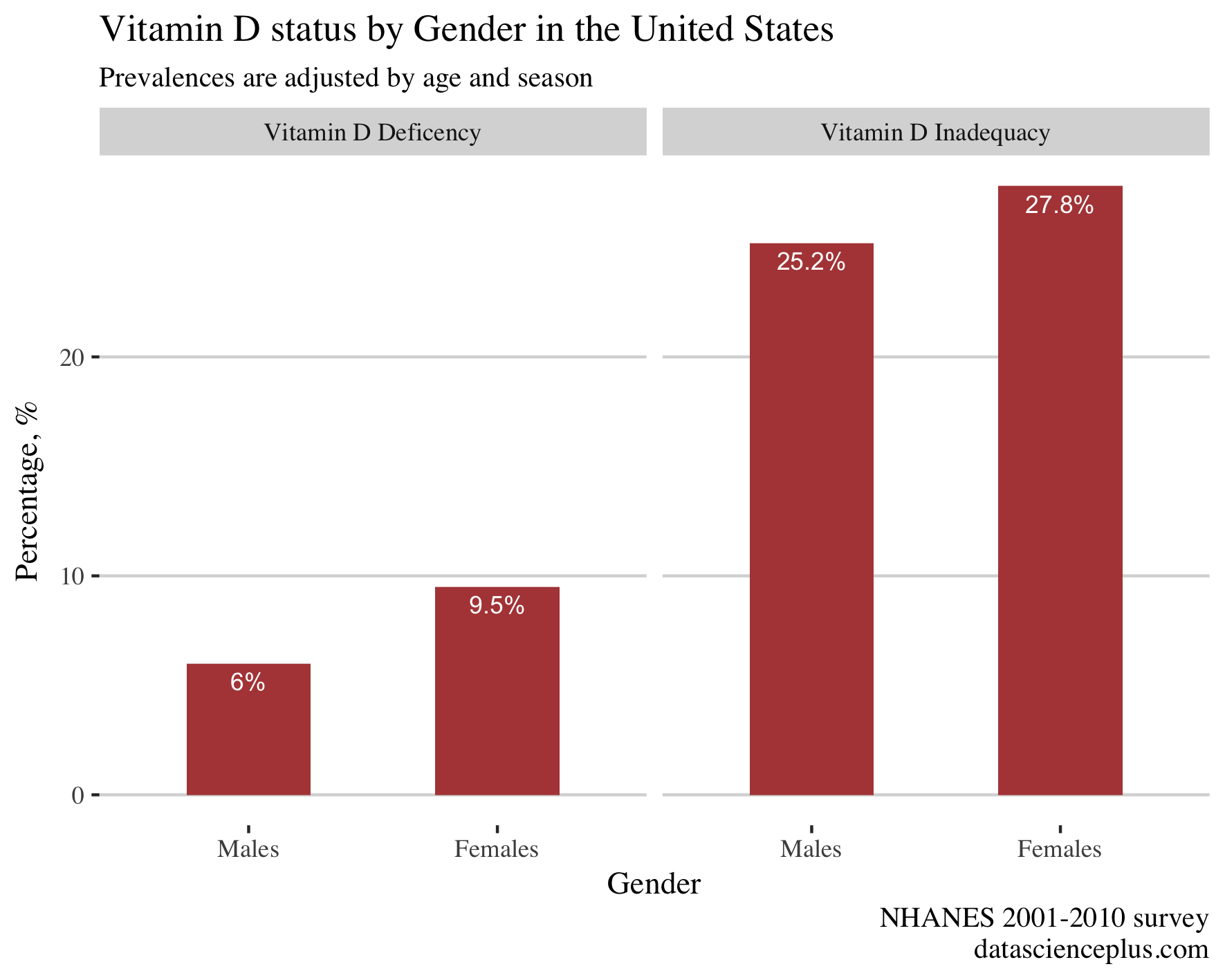
Vitamin D inadequacy and deficiency differed by gender and it was lower in males than females.
Prevalences of Vitamin D status by race
Given that vitamin D is produced in the skin, I calculated the status of vitamin D by ethnicity.
reg_dat %>%
  group_by(race) %>%
  summarise(
    "Vitamin D Deficency" = round(mean(adj_vitD_defi), 1),
    "Vitamin D Inadequacy" = round(mean(adj_vitD_inad), 1)
    ) %>%
  gather("Vitamin D", "%", -race) %>%
  ggplot(., aes(x=race, y=`%`)) +
  geom_bar(stat = "identity", width = 0.7, fill = "#B24745") +
  geom_text(aes(label = paste0(`%`, "%"), y = `%`),
            vjust = 1.5, size = 3, color = "#FFFFFF") +
  facet_grid(~`Vitamin D`) +
  theme_hc() +
  theme(text = element_text(family = "serif", size = 11), legend.position="none",
        axis.text.x = element_text(angle = 45, hjust = 1)) +
  labs(
    title = "Vitamin D status by Race in the United States",
    subtitle = "Prevalences are adjusted by age and season",
    caption = "NHANES 2001-2010 survey\ndatascienceplus.com",
    x = "Race",
    y = "Percentage, %"
    )
This gives the plot:
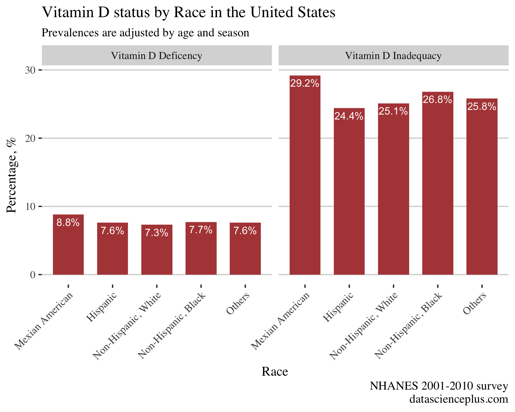
The prevalence of vitamin D inadequacy was higher in Mexican American and lowest in the non-Hispanic white ethnicity.
Prevalences of Vitamin D status by pregnancy status
In this analysis, I will include only females in reproductive age (14 to 44 years)
reg_dat %>%
  filter(gender == "Females", RIDAGEYR > 14, RIDAGEYR < 44) %>%
  group_by(pregnancy) %>%
  summarise(
    "Vitamin D Deficency" = round(mean(adj_vitD_defi), 1),
    "Vitamin D Inadequacy" = round(mean(adj_vitD_inad), 1)
    ) %>%
  gather("Vitamin D", "%", -pregnancy) %>%
  ggplot(., aes(x=pregnancy, y=`%`)) +
  geom_bar(stat = "identity", width = 0.7, fill = "#B24745") +
  geom_text(aes(label = paste0(`%`, "%"), y = `%`),
            vjust = 1.5, size = 3, color = "#FFFFFF") +
  facet_grid(~`Vitamin D`) +
  theme_hc() +
  theme(text = element_text(family = "serif", size = 11), legend.position="none") +
  labs(
    title = "Vitamin D status by Pregnancy in the United States",
    subtitle = "Prevalences are adjusted by age and season",
    caption = "NHANES 2001-2010 survey\ndatascienceplus.com",
    x = "Pregnancy Status",
    y = "Percentage, %"
    )
The plot is shown below:
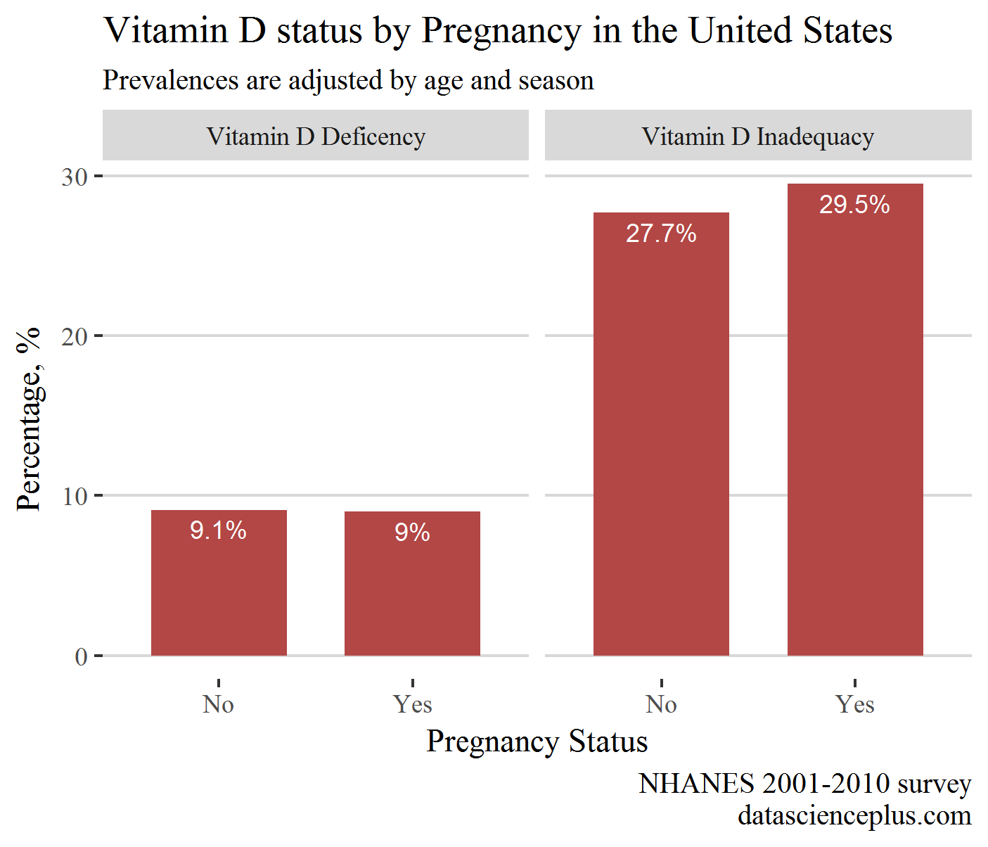
Surprising, the prevalence of inadequacy was higher in pregnant females than in non-pregnant.
Vitamin D trends from 2001-2010
Now I will build the age and season-adjusted trajectories of prevalences of vitamin D deficiency and inadequacy in NHANES 2001-2010. This analysis will be gender specific.
reg_dat %>%
  group_by(wave, gender) %>%
  summarise_at(vars(adj_vitD_inad, adj_vitD_defi), funs(mean)) %>%
  gather("VitaminD", "%", -wave, -gender) %>%
  mutate(VitaminD = if_else(VitaminD == "adj_vitD_inad", "Inadequacy", "Deficiency")) %>%
  ggplot(aes(wave, `%`, fill = VitaminD, group = VitaminD)) +
  geom_line(color = "black", size = 0.3) +
  geom_point(colour="black", pch=21, size = 3) +
  facet_grid(~gender) +
  scale_fill_jama() +
  theme_hc() +
  theme(text = element_text(family = "serif", size = 11), legend.position="bottom") +
  labs(
    title = "Trends of vitamin D in the United States",
    subtitle = "Prevalences are adjusted by age and season",
    caption = "NHANES 2001-2010 survey\ndatascienceplus.com",
    x = "Survey Cycle Years",
    y = "Percentage, %",
    fill = "Vitamin D Status"
    ) +
  scale_y_continuous(limits=c(0,40), breaks=seq(0,40, by = 5))
This gives the plot:
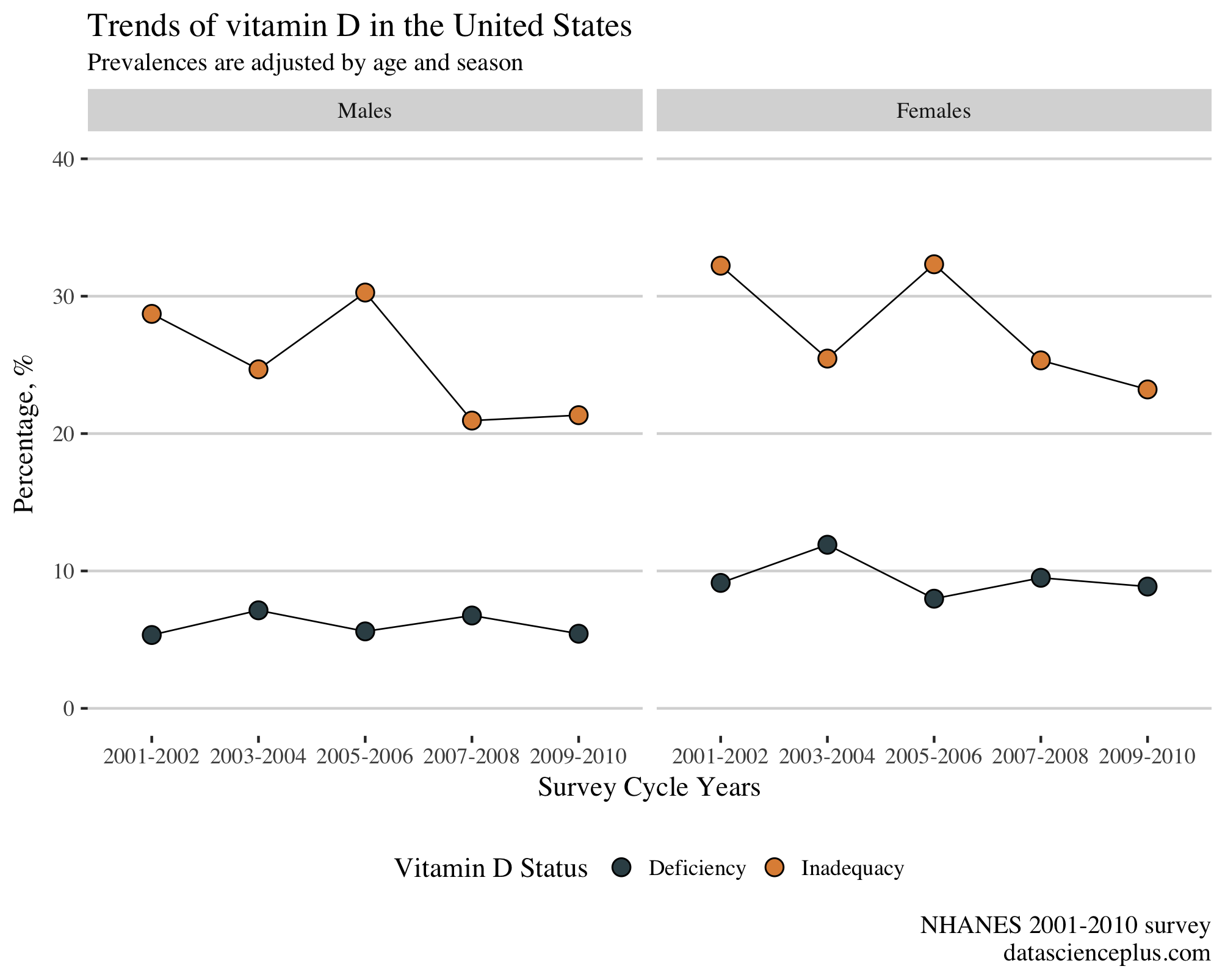
From 2001 to 2010 there is a drop in the prevalence of vitamin D inadequacy in males and females in the US. While the prevalence of deficiency remains stable over the years in both genders, females have a higher prevalence of deficiency compared to males.
I look forward to hearing any feedback or questions.