Time series data are data points collected over a period of time as a sequence of time gap. Time series data analysis means analyzing the available data to find out the pattern or trend in the data to predict some future values which will, in turn, help more effective and optimize business decisions.
Methods for time series analysis
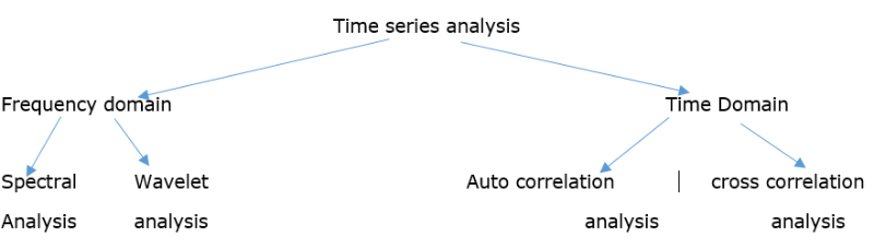
Moreover, time series analysis can be classified as:
- 1. Parametric and Non-parametric
- 2. Linear and Non-linear and
- 3. Univariate and multivariate
Techniques used for time series analysis:
- 1. ARIMA models
- 2. Box-Jenkins multivariate models
- 3. Holt winters exponential smoothing (single, double and triple)
ARIMA modeling
ARIMA is the abbreviation for AutoRegressive Integrated Moving Average. Auto Regressive (AR) terms refer to the lags of the differenced series, Moving Average (MA) terms refer to the lags of errors and I is the number of difference used to make the time series stationary.
Assumptions of ARIMA model
- 1. Data should be stationary – by stationary it means that the properties of the series doesn’t depend on the time when it is captured. A white noise series and series with cyclic behavior can also be considered as stationary series.
- 2. Data should be univariate – ARIMA works on a single variable. Auto-regression is all about regression with the past values.
Steps to be followed for ARIMA modeling:
- 1. Exploratory analysis
- 2. Fit the model
- 3. Diagnostic measures
The first step in time series data modeling using R is to convert the available data into time series data format. To do so we need to run the following command in R:
tsData = ts(RawData, start = c(2011,1), frequency = 12)
where RawData is the univariate data which we are converting to time series. start gives the starting time of the data, in this case, its Jan 2011. As it is a monthly data so ‘frequency=12’.
This is how the actual dataset looks like:
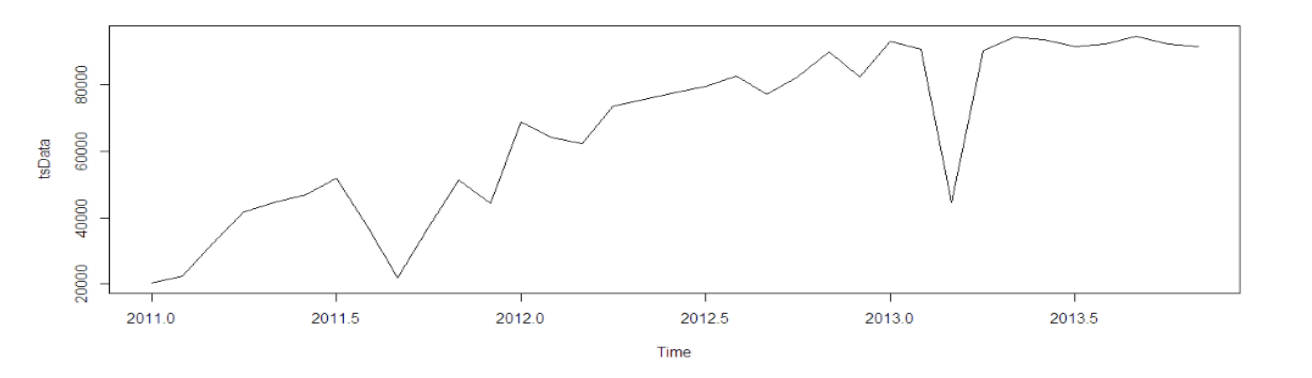
We can infer from the graph itself that the data points follows an overall upward trend with some outliers in terms of sudden lower values. Now we need to do some analysis to find out the exact non-stationary and seasonality in the data.
Exploratory analysis
- 1. Autocorrelation analysis to examine serial dependence: Used to estimate which value in the past has a correlation with the current value. Provides the p,d,q estimate for ARIMA models.
- 2. Spectral analysis to examine cyclic behavior: Carried out to describe how variation in a time series may be accounted for by cyclic components. Also referred to as a Frequency Domain analysis. Using this, periodic components in a noisy environment can be separated out.
- 3. Trend estimation and decomposition: Used for seasonal adjustment. It seeks to construct, from an observed time series, a number of component series(that could be used to reconstruct the original series) where each of these has a certain characteristic.
Before performing any EDA on the data, we need to understand the three components of a time series data:
- Trend: A long-term increase or decrease in the data is referred to as a trend. It is not necessarily linear. It is the underlying pattern in the data over time.
- Seasonal: When a series is influenced by seasonal factors i.e. quarter of the year, month or days of a week seasonality exists in the series. It is always of a fixed and known period. E.g. – A sudden rise in sales during Christmas, etc.
- Cyclic: When data exhibit rises and falls that are not of the fixed period we call it a cyclic pattern. For e.g. – duration of these fluctuations is usually of at least 2 years.
We can use the following R code to find out the components of this time series:
components.ts = decompose(tsData)
plot(components.ts)
The output will look like this:
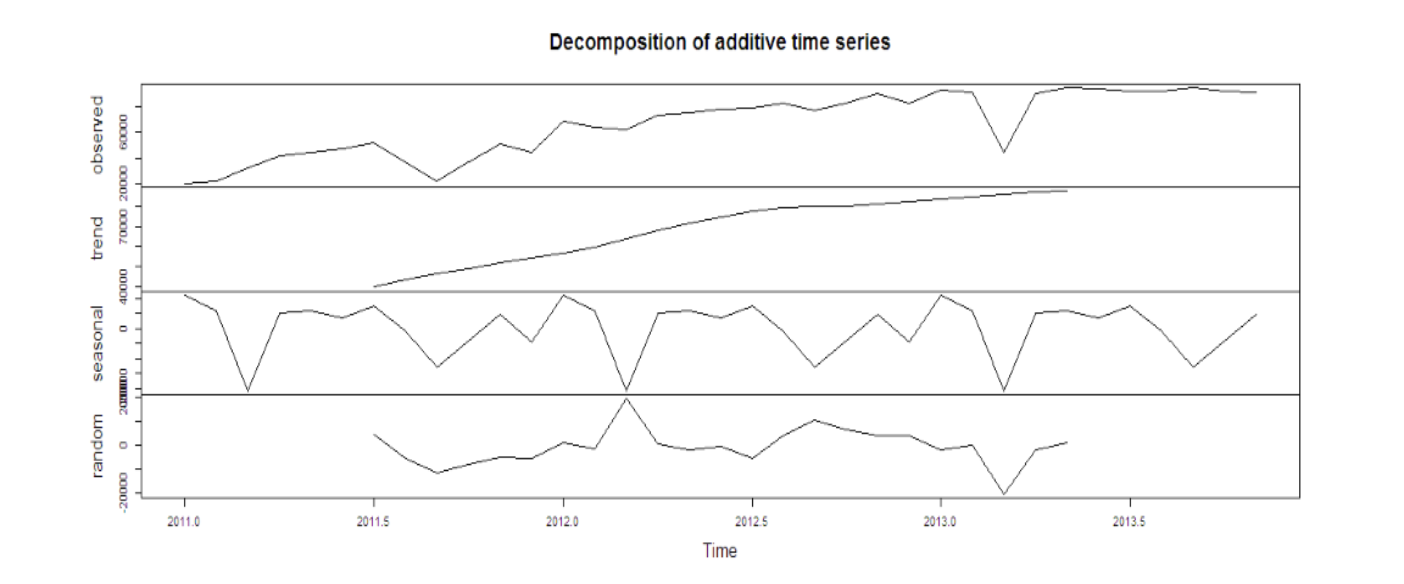
Here we get 4 components:
- Observed – the actual data plot
- Trend – the overall upward or downward movement of the data points
- Seasonal – any monthly/yearly pattern of the data points
- Random – unexplainable part of the data
Observing these 4 graphs closely, we can find out if the data satisfies all the assumptions of ARIMA modeling, mainly, stationarity and seasonality.
Next, we need to remove non-stationary part for ARIMA. For the sake of discussion here, we will remove the seasonal part of the data as well. The seasonal part can be removed from the analysis and added later, or it can be taken care of in the ARIMA model itself.
To achieve stationarity:
- difference the data – compute the differences between consecutive observations
- log or square root the series data to stabilize non-constant variance
- if the data contains a trend, fit some type of curve to the data and then model the residuals from that fit
- Unit root test – This test is used to find out that first difference or regression which should be used on the trending data to make it stationary. In Kwiatkowski-Phillips-Schmidt-Shin (KPSS) test, small p-values suggest differencing is required.
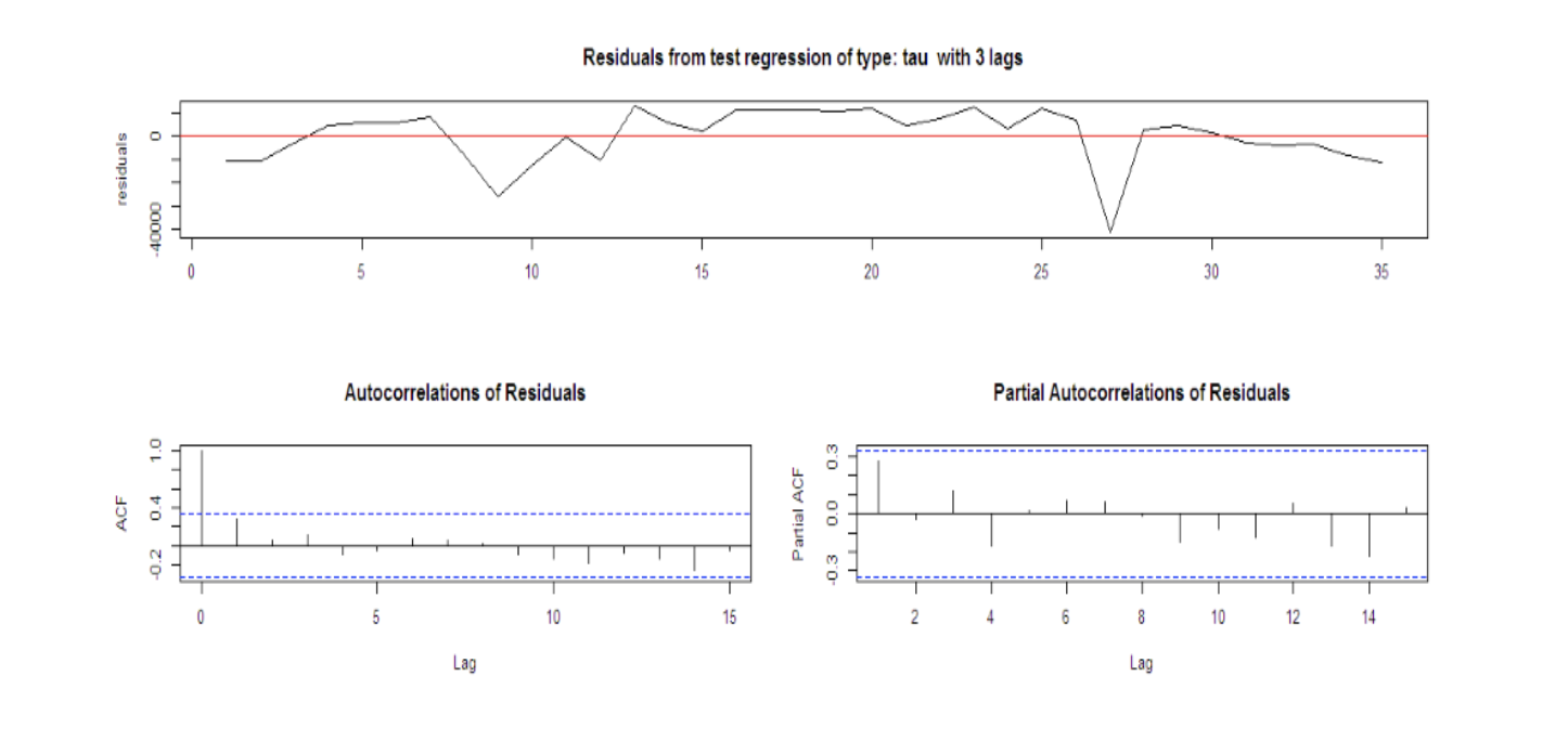
The R code for unit root test:
library("fUnitRoots")
urkpssTest(tsData, type = c("tau"), lags = c("short"),use.lag = NULL, doplot = TRUE)
tsstationary = diff(tsData, differences=1)
plot(tsstationary)
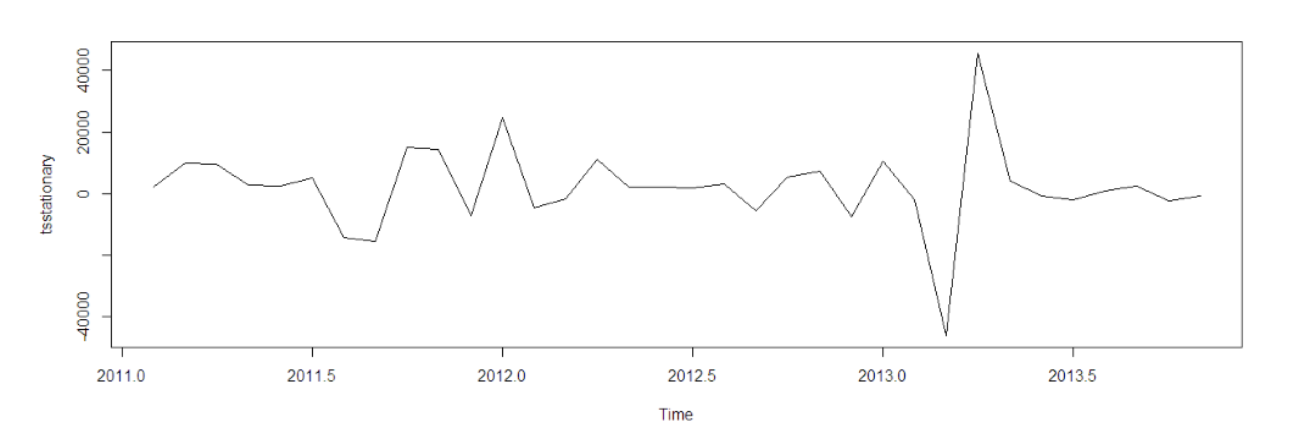
The output will look like this:
After removing non-stationarity:
Various plots and functions that help in detecting seasonality:
- A seasonal subseries plot
- Multiple box plot
- Auto correlation plot
ndiffs()is used to determine the number of first differences required to make the time series non-seasonal
R codes to calculate autocorrelation:
acf(tsData,lag.max=34)
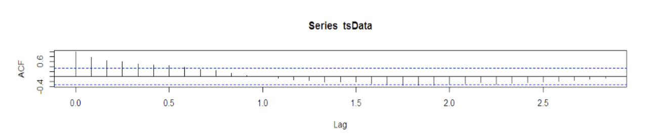
The autocorrelation function (acf()) gives the autocorrelation at all possible lags. The autocorrelation at lag 0 is included by default which always takes the value 1 as it represents the correlation between the data and themselves. As we can infer from the graph above, the autocorrelation continues to decrease as the lag increases, confirming that there is no linear association between observations separated by larger lags.
timeseriesseasonallyadjusted <- tsData- timeseriescomponents$seasonal
tsstationary <- diff(timeseriesseasonallyadjusted, differences=1)
To remove seasonality from the data, we subtract the seasonal component from the original series and then difference it to make it stationary.
After removing seasonality and making the data stationary, it will look like:

Smoothing is usually done to help us better see patterns, trends in time series. Generally it smooths out the irregular roughness to see a clearer signal. For seasonal data, we might smooth out the seasonality so that we can identify the trend. Smoothing doesn’t provide us with a model, but it can be a good first step in describing various components of the series.
To smooth time series:
-
Ordinary moving average (single, centered) – at each point in time we determine averages of observed values that precede a particular time.
To take away seasonality from a series, so we can better see a trend, we would use a moving average with a length = seasonal span. Seasonal span is the time period after which a seasonality repeats, e.g. – 12 months if seasonality is noticed every December. Thus in the smoothed series, each smoothed value has been averaged across the complete season period. - Exponentially weighted average – at each point of time, it applies weighting factors which decrease exponentially. The weighting for each older datum decreases exponentially and never reaching zero.
Fit the model
Once the data is ready and satisfies all the assumptions of modeling, to determine the order of the model to be fitted to the data, we need three variables: p, d, and q which are non-negative integers that refer to the order of the autoregressive, integrated, and moving average parts of the model respectively.
To examine which p and q values will be appropriate we need to run acf() and pacf() function.
pacf() at lag k is autocorrelation function which describes the correlation between all data points that are exactly k steps apart- after accounting for their correlation with the data between those k steps. It helps to identify the number of autoregression (AR) coefficients(p-value) in an ARIMA model.
The R code to run the acf() and pacf() commands.
acf(tsstationary, lag.max=34)
pacf(tsstationary, lag.max=34)
The plots will look like:

Shape of acf() to define values of p and q:
Looking at the graphs and going through the table we can determine which type of the model to select and what will be the values of p, d and q.

fitARIMA <- arima(tsData, order=c(1,1,1),seasonal = list(order = c(1,0,0), period = 12),method="ML")
library(lmtest)
coeftest(fitARIMA)
order specifies the non-seasonal part of the ARIMA model: (p, d, q) refers to the AR order, the degree of difference, and the MA order.
seasonal specifies the seasonal part of the ARIMA model, plus the period (which defaults to frequency(x) i.e 12 in this case). This function requires a list with components order and period, but given a numeric vector of length 3, it turns them into a suitable list with the specification as the ‘order’.
method refers to the fitting method, which can be ‘maximum likelihood(ML)’ or ‘minimize conditional sum-of-squares(CSS)’. The default is conditional-sum-of-squares.
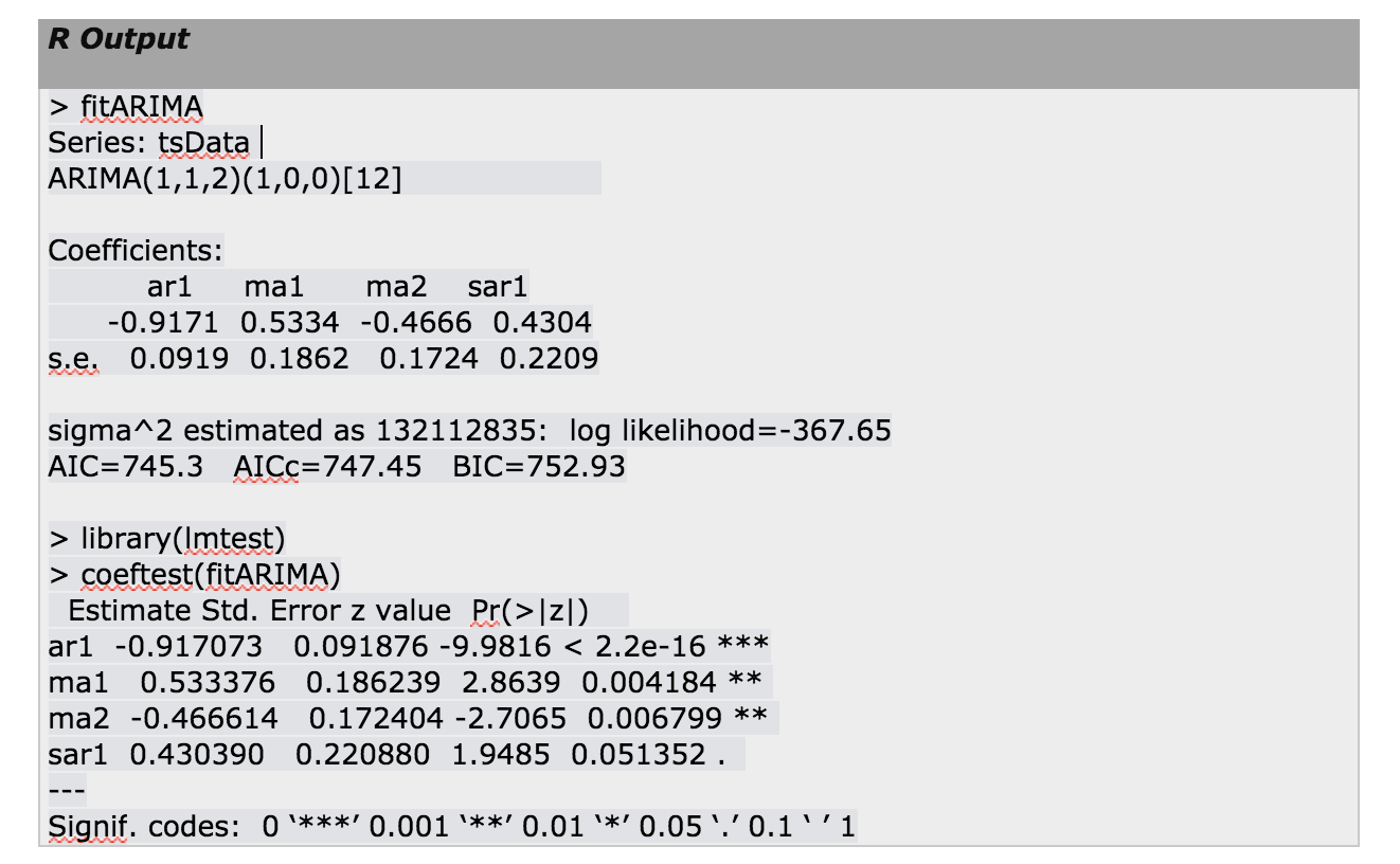
This is a recursive process and we need to run this arima() function with different (p,d,q) values to find out the most optimized and efficient model.
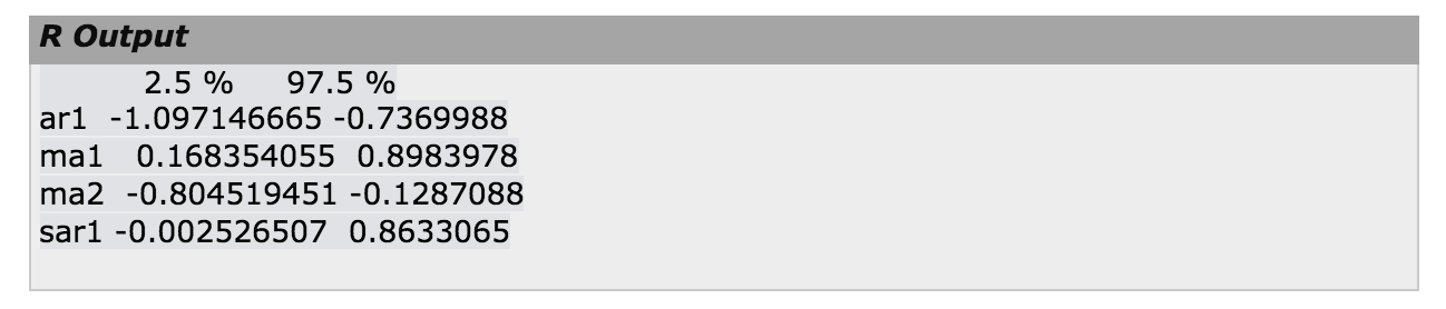
The output from fitarima() includes the fitted coefficients and the standard error (s.e.) for each coefficient. Observing the coefficients we can exclude the insignificant ones. We can use a function confint() for this purpose.
We can use a function confint() for this purpose.
confint(fitARIMA)
Choosing the best model
R uses maximum likelihood estimation (MLE) to estimate the ARIMA model. It tries to maximize the log-likelihood for given values of p, d, and q when finding parameter estimates so as to maximize the probability of obtaining the data that we have observed.
Find out Akaike’s Information Criterion (AIC) for a set of models and investigate the models with lowest AIC values. Try Schwarz Bayesian Information Criterion (BIC) and investigate the models with lowest BIC values. When estimating model parameters using maximum likelihood estimation, it is possible to increase the likelihood by adding additional parameters, which may result in over fitting. The BIC resolves this problem by introducing a penalty term for the number of parameters in the model. Along with AIC and BIC, we also need to closely watch those coefficient values and we should decide whether to include that component or not according to their significance level.
Diagnostic measures
Try to find out the pattern in the residuals of the chosen model by plotting the ACF of the residuals, and doing a portmanteau test. We need to try modified models if the plot doesn’t look like white noise.
Once the residuals look like white noise, calculate forecasts.
Box-Ljung test
It is a test of independence at all lags up to the one specified. Instead of testing randomness at each distinct lag, it tests the "overall" randomness based on a number of lags, and is therefore a portmanteau test. It is applied to the residuals of a fitted ARIMA model, not the original series, and in such applications the hypothesis actually being tested is that the residuals from the ARIMA model have no autocorrelation.
R code to obtain the box test results:
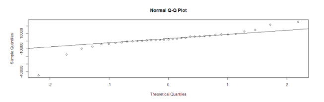
acf(fitARIMA$residuals)
library(FitAR)
boxresult-LjungBoxTest (fitARIMA$residuals,k=2,StartLag=1)
plot(boxresult[,3],main= "Ljung-Box Q Test", ylab= "P-values", xlab= "Lag")
qqnorm(fitARIMA$residuals)
qqline(fitARIMA$residuals)
Output:
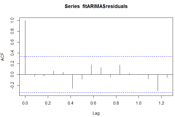
The ACF of the residuals shows no significant autocorrelations.

The p-values for the Ljung-Box Q test all are well above 0.05, indicating “non-significance.”
The values are normal as they rest on a line and aren’t all over the place.
As all the graphs are in support of the assumption that there is no pattern in the residuals, we can go ahead and calculate the forecast.
Work flow diagram

auto.arima() function:
The forecast package provides two functions: ets() and auto.arima() for the automatic selection of exponential and ARIMA models.
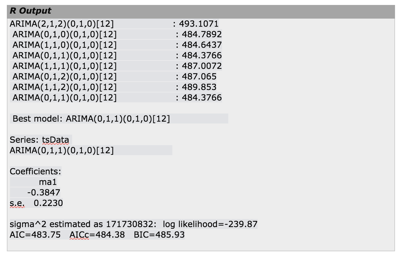
The auto.arima() function in R uses a combination of unit root tests, minimization of the AIC and MLE to obtain an ARIMA model.
KPSS test is used to determine the number of differences (d) In Hyndman-Khandakar algorithm for automatic ARIMA modeling.
The p,d, and q are then chosen by minimizing the AICc. The algorithm uses a stepwise search to traverse the model space to select the best model with smallest AICc.
If d=0 then the constant c is included; if d≥1 then the constant c is set to zero. Variations on the current model are considered by varying p and/or q from the current model by ±1 and including/excluding c from the current model.
The best model considered so far (either the current model, or one of these variations) becomes the new current model.
Now, this process is repeated until no lower AIC can be found.
auto.arima(tsData, trace=TRUE)
Forecasting using an ARIMA model
The parameters of that ARIMA model can be used as a predictive model for making forecasts for future values of the time series once the best-suited model is selected for time series data.
The d-value effects the prediction intervals —the prediction intervals increases in size with higher values of ‘d’. The prediction intervals will all be essentially the same when d=0 because the long-term forecast standard deviation will go to the standard deviation of the historical data.
There is a function called predict() which is used for predictions from the results of various model fitting functions. It takes an argument n.ahead() specifying how many time steps ahead to predict.
predict(fitARIMA,n.ahead = 5)
forecast.Arima() function in the forecast R package can also be used to forecast for future values of the time series. Here we can also specify the confidence level for prediction intervals by using the level argument.
futurVal <- forecast.Arima(fitARIMA,h=10, level=c(99.5))
plot.forecast(futurVal)
We need to make sure that the forecast errors are not correlated, normally distributed with mean zero and constant variance. We can use the diagnostic measure to find out the appropriate model with best possible forecast values.
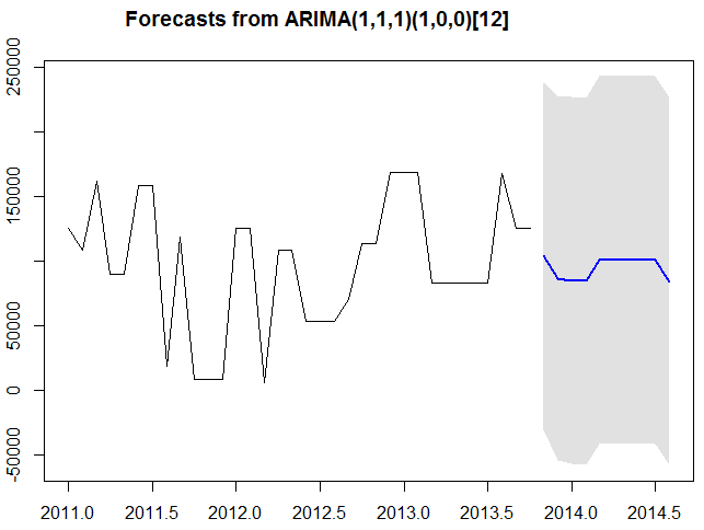
The forecasts are shown as a blue line, with the 80% prediction intervals as a dark shaded area, and the 95% prediction intervals as a light shaded area.
This is the overall process by which we can analyze time series data and forecast values from existing series using ARIMA.
Click here to get the entire code.
The function urkpssTest for stationary cannot be found in R. Any help plz ???
https://uploads.disquscdn.com/images/d4f79881d53549c0a7e5eb07811c2000c9fc213a69ff03edb328d3611fe8ca59.png
function urkpssTest for stationary cannot be found in R. Any help plz ???
Hi, I am kind of stuck at the step where I am trying to forecast using the forecast.Arima function. But there’s an error “the function does not exist”?. Can you please let me know why this is happening?
instal.packages(“forecast”)
librarie(forecast)
You need to add “forecast” library with the code above.
install.packages(“forecast”)
librarie(forecast)
https://uploads.disquscdn.com/images/d4f79881d53549c0a7e5eb07811c2000c9fc213a69ff03edb328d3611fe8ca59.png The function urkpssTest for stationary cannot be found in R. Any help plz ???
This is a very informative article. What is boxresult? I do not understand what this is or where it is defined. Someone please help.
Excellent resource. I have a lot of the background conceptual knowledge but just didn’t know how to pull it all together in R. This helps me along a lot.
What is the value of ‘timeseriescomponents$seasonal’ ?
It is not defined in code. Please help.
My bad Shashi! timeseriescomponents$seasonal is components.ts$seasonal. If you want to replicate the code please use the entire code from my GitHub profile linked along with this article.
Thank you Subhasree!!
You have mentioned in your previous comment that you will include results of codes. Is this code is not enough or we have to add more to this?
Hi
Thanks for the article, how we do this for multiple data. for example 10 centers or 10 stores. thanks
If I understand your question correctly you may want to build separate models for each store as their historical data must be different from each other
Hello Subhasree
I have the same question what you understood
Hi, I thought the article was extremely informative. I am currently modeling vehicle sales. I have done all steps, but in my forecasting course we need to add the seasonality back using seasonal dummies. I have done this, using XREG. However, my model does not work. Is there a way of adding seasonal back in the arima model without using the seasonal list order?
Thank you Philip. This is an interesting use case. Xreg should have worked. Can you elaborate what error you are getting? Are you facing something like this? https://github.com/robjhyndman/forecast/issues/682
You can also try Arimax if you have the seasonal dummies as independent variables.
Hope this helps
Are you really confident to your assumptions of ARIMA Model? Where did you get them? All of them, i suppose, has been written by not looking any basic econometrics books, since they are completely wrong.
If they are completely wrong why don’t you enlighten us by telling what the right ones are?
As I have mentioned before as well, this article is just my view and my research and the way I learnt about ARIMA. I am not claiming to know everything or know the best anywhere. If you know more/better, please share it with the audience.
where can we get the data.csv, please?
Unfortunately Kevin I don’t have the data.csv anymore with me as it has been years since I first wrote this article. It was a simple dataset with just 2 columns one for date and other for numbers, so you can really just create a dummy dataset in excel and play with the code.
After reading the articles, the following points needs to be cleared:
1. In the entire post, there is no single results displayed. However, theoretically there are many results which are mandatory for any time series econometrics analysis.
2. Graphical analysis will give us only the indication of the trend of the data which are confirmed by some tests.
3. In the first graph, there is no clear upward trend in the data, but it was mentioned that ‘data shows upward trend’. In fact, the graphs indicates a stationary series. If ADF test will confirm it. Though KPSS test command is given ; but results are missing.
4. Lag selection method also not clarified which is very important.
5. The overall methods is not looking very solid as far as the concepts/writing from some good books on Time Series Econometrics such as Walter Enders, Greene etc.
6. Finally the packages used are not the best. There are other very good packages and functions in R to conduct ARIMA.
Thank you for your feedback Bidyut. 1st of all I am not claiming this is the best method to do time series analysis in R. This is just my view and my research and the way I learnt about ARIMA. Obviously people who have written a book about it will know more than me! This was my way of sharing everything I know about time series, so that people who have just started learning can get a comprehensive idea on the topic. If there is any mistake or ways to make this article better I will be more than happy to modify it.
As you mentioned, I will include the results of the codes and clarify if something is not very clear.