In this article I am going to talk about the non-parametric techniques used for survival analysis. To comprehend this article effectively, you’ll need basic understanding of probability, statistics and R. If you have any questions regarding the concept or the code, feel free to comment, I’ll be more than happy to get back to you.
Survival analysis is a set of methods to analyze the ‘time to occurrence’ of an event. The response is often referred to as a failure time, survival time, or event time. These methods are widely used in clinical experiments to analyze the ‘time to death’, but nowadays these methods are being used to predict the ‘when’ and ‘why’ of customer churn or employee turnover as well.
The dependent variables for the analysis are generally two functions:
Survival Function: It is the probability that an individual survives beyond a specific time T. It has the following properties:
- It is non-increasing
- At time t = 0, S(t) = 1. In other words, the probability of surviving past time 0 is 1
- At time t = ∞, S(t) = S(∞) = 0. As time goes to infinity, the survival curve goes to 0
In theory, the survival function is smooth. In practice, events are observed on a discrete time scale
Hazard Function: the probability of failure in an infinitesimally small time period given that the individual has survived up till the present time. The cumulative hazard describes the accumulated risk up to the present time.
To estimate these two functions, three types of analysis are generally performed:
- Non-parametric
- Semi-parametric
- Parametric
Censoring of Data
The observed data in this type of analysis is generally consisted of a binary event variable (event occurred =1) and a ‘time to the event’ variable. In some observations the time to event variable can be blank if the participants drop out before the study ends or the participants are event free at the end of the observation period. Those types of observations are called censored.
Censoring can be of two types:
Right Censoring: where the time of event is unknown when the subject is removed from the study or the time of event is after the end of the study. There can be three types of Right Censoring:
- Fixed Type I Censoring: occurs when a study is designed to end after C years of follow up. In this case everyone who doesn’t have an event observed during the course of the study is censored at C years
- Random Type I Censoring: the study is designed to end after C years, but censored subjects don’t have the same censoring type
- Type II Censoring: a study ends when there is a pre-specified number of events
Left Censoring: where the subject’s survival time is incomplete on the left side of the follow up period e.g. the exact time of exposure is unknown
The same observation can be both left and right censored, termed as interval censoring.
Only one condition of censoring is that it must be independent of the event being looked at. Otherwise the estimates of the survival distribution can be seriously biased. This is called non-informative censoring.
Why not Linear Regression?
Survival times are typically positive numbers, ordinary linear regression may not be the best choice unless these times are first transformed in a way that removes this restriction
OLS can’t handle censoring of observations effectively
Difference between Logistic Regression and Survival Analysis:

Non-parametric Method (Kaplan Meier Estimate)
The Kaplan-Meier survival curve is defined as the probability of surviving in a given length of time while considering time in many small intervals.
There are three assumptions used in this analysis:
- At any time records which are censored have the same survival prospects as those who continue to be followed
- Survival probabilities are the same for subjects recruited early and late in the study
- Event happens at the time specified
The Kaplan-Meier estimate is also called as “product limit estimate”. It involves computing of probabilities of occurrence of an event at a certain point of time. These successive probabilities are multiplied by any earlier computed probabilities to get the final estimate.
For each time interval, survival probability is calculated as the number of subjects surviving divided by the number of patients at risk. Subjects who have died, dropped out, or move out are not counted as “at risk” i.e., subjects who are lost are considered “censored” and are not counted in the denominator. Total probability of survival till that time interval is calculated by multiplying all the probabilities of survival at all time intervals preceding that time.
Comparing multiple Survival Curves
Curves for two different groups of subjects can be compared. We can look for gaps in these curves in a horizontal or vertical direction. A vertical gap means that at a specific time point, one group had a greater fraction of subjects surviving. A horizontal gap means that it took longer for one group to experience a certain fraction of deaths.
The two survival curves can be compared statistically by testing the null hypothesis i.e. there is no difference regarding survival among two interventions. This null hypothesis is statistically tested by another test known as log-rank test.
Log-Rank Test
The log-rank test is the most commonly-used statistical test for comparing the survival distributions of two or more groups.
The null hypothesis is that the hazard rates of all populations are equal at all times less than the maximum observed time and the alternative hypothesis is that at least two of the hazard rates are different at some time less than the observed maximum time.
The test statistic is:
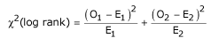
where the O1 and O2 are the total numbers of observed events in groups 1 and 2, respectively, and E1 and E2 the total numbers of expected events.
The total expected number of events for a group is the sum of the expected number of events at the time of each event. The expected number of events at the time of an event can be calculated as the risk for death at that time multiplied by the number alive in the group. Under the null hypothesis, the risk of death (number of deaths/number alive) can be calculated from the combined data for both groups.
The test statistic is compared with a χ2 distribution with 1 degree of freedom.
It has the considerable advantage that it does not require us to know anything about the shape of the survival curve or the distribution of survival times.
The log-rank test is based on the same assumptions as the Kaplan Meier survival curve – namely, that censoring is unrelated to prognosis, the survival probabilities are the same for subjects recruited early and late in the study, and the events happened at the times specified.
The log-rank test is most likely to detect a difference between groups when the risk of an event is consistently greater for one group than another. It is unlikely to detect a difference when survival curves cross.
These tests are very useful in assessing whether a covariate affects survival. However, they do not allow us to say how survival is affected. Ideally, we’d like to be able to say how much more at risk on group is than another. This can be done using Cox’s proportional hazards model, a semi-parametric model to investigate the functional relationship between the covariates and survival.
Pointwise Confidence Intervals of Survival
A pointwise confidence interval for the survival probability at a specific time t is represented by two confidence limits which have been constructed so that the probability that the true survival probability lies between them is 1− α. These limits are constructed for a single time point. Several of them cannot be used together to form a confidence band such that the entire survival function lies within the band. When these are plotted with the survival curve, these limits must be interpreted on an individual, point by point, basis.
Three difference confidence intervals are available. All three confidence intervals perform about the same in large samples. The linear (Greenwood) interval is the most commonly used. However, the log-transformed and the arcsine-square intervals behave better in small to moderate samples, so they are recommended.
Kaplan Meier Estimate in R
To create a survival object:
Surv(time, time2, event)
where, time is for right censored data
time2 is ending time of the interval for interval censored or counting process data only
type is a character string specifying the type of censoring.
When the type argument is missing the code assumes a type based on the following rules:
- If there are two unnamed arguments, they will match time and event in that order. If there are three unnamed arguments they match time, time2 and event
- If the event variable is a factor then type ‘mstate’ is assumed. Otherwise type ‘right’ if there is no time2 argument, and type ‘counting’ if there is
To create survival curves:
survfit( formula)
where, formula has a Surv object as the response on the left of the ~ operator and for a single survival curve the right hand side should be ~ 1.
For eg.
model<- survfit(Surv(time,event) ~ 1)
For multiple survival curves, the right hand side can be the variable to differentiate survival functions
For eg.
model<- survfit(Surv(time,event) ~ group)
To plot the survival curve:
Plot(survfit( formula))
To understand if there is a statistical difference between two survival curves:
survdiff(survival ~ group, rho=0)
where rho a scalar parameter that controls the type of test. With rho = 0 this is the log-rank or Mantel-Haenszel test, and with rho = 1 it is equivalent to the Peto & Peto modification of the Gehan-Wilcoxon test.
To give greater weight to the first part of the survival curves, use rho larger than 0. To give weight to the later part of the survival curves, use rho smaller than 0.
For a detailed example of the above functions, please have a look at the this link.
In a future article, I’ll discuss semi-parametric i.e cox proportional hazard model and parametric models for survival analysis.
References:
Thank you for this article. It was easy to read, understand and apply. I have one question:
Where you stated “To give greater weight to the first part of the survival curves, use rho larger than 0. To give weight to the later part of the survival curves, use rho smaller than 0” under estimating the KM.
Why would you give greater weight to one section than another? I am applying survival analysis to seedling fate so I guess an answer in that context if applicable would help me to understand. can this weighting be useful when the subjects have entered the study at different time points (i.e. planted in 2 different years, the study runs for 24 mo total)?
Cheers, any help appreciated
J
Hey Jessica, thanks for reading my article. The situation of giving different weights come when you have non-proportional hazards. If you feel the earlier difference in your survival curves is more meaningful than your later difference, you may use the rho value accordingly.