Naïve Bayes is a probability machine learning algorithm which is used in multiple classification tasks. In this article, I’m going to present a complete overview of the Naïve Bayes algorithm and how it is built and used in real-world.
- Overview
- Concept of conditional probability
- Bayes Rule
- Naïve Bays and example
- Laplace correction
- Gaussian Naïve Bayes
- Creating a Naïve Bayes classifier (Python)
- How to improve your model
Overview
Naive Bayes is a probabilistic machine learning algorithm designed to accomplish classification tasks. It is currently being used in varieties of tasks such as sentiment prediction analysis, spam filtering and classification of documents etc.
Here the word naïve represents that the features which undergo into the model are independent to one another. Suppose if the value of one feature gets changed then it will not directly affect the value of other feature used in the algorithm.
Now you must be thinking why Naive Bayes (NB) is so much popular?
The main reason behind its popularity is that it can be written into the code very easily delivering predictions model in very less time. Thus it can be used in the real-time model predictions. Its scalable feature allows organizations to implement it in their application for providing quick solutions to the user’s request.
Now since you are here to understand the Naive Bayes working. It requires a clear understanding of conditional probability which is the backbone of this algorithm.
Conditional Probability
What will be the probability of getting 5 when you roll dice of six faces? Well, it would be 1/6 which comes to 0.166. Similarly, when you flip a coin during the match for toss there is an equal probability of getting heads or tails. So you can say the probability of a tail is going to be 50%.
Now, let’s understand it with the help of a playing card deck. Suppose you took a card from the deck so what will be the probability of getting a king card? The given card is a spade. Since I have already discussed it is spade so the denominator or eligibility of the population would be 13 rather than 52. Since only 1 king will all under a spade so the probability of getting a king card will be 1/13 which comes out to be 0.077.
It is the best example of conditional probability. In mathematics, the conditional probability of X over given Y is computed by:
P(X|Y)=P(X & Y)/P(B)
It seems very easy to calculate but when it comes to complex situations the scenario gets a little difficult. Let’s understand it with the help of an example.
Consider a company with a total population of 100. There are 100 persons who can be assistant manager, senior manager, manager etc. Or it can be the population of male and female employees.
With the below-described table of 100 persons, you can calculate the conditional probability of a particular member who is a senior manager and a female.
Conditional Probability
| S.No | Male | Female | Total |
| Senior Manager | 9 | 11 | 20 |
| Assistant Manager | 30 | 50 | 80 |
| Total | 39 | 61 | 100 |
For calculating the above-discussed figure, you can make a filter for the female sub-population of 61 and work on 11 female senior managers.
The conditional probability will be
P (Senior Manager| Female)= P (Senior Manager Π Female) / P (Female) = 11/61 = 0.18
It can be represented as the intersection of Senior Manager (X) and Female (Y) which is divided by Female(Y). The Naïve Bayes rule is computed from these two equations
P (X | Y) = P (X Π Y) / P (Y) …….(1)
P (Y | X) = P (X Π Y) / P (X) .……(2)
Bayes Rule:
The Bayes rule is a concept of determining P (W | Z) from the provided training datasets which are P (Z | W). To find it, we will replace the X and Y in the above equation with the feature and response which is W and Z respectively.
For test observation, W would be known and Z will be unknown. To calculate each row from the test data set you will calculate the probability of Z and consider W event has already happened.
Now, what will happen when Z will have more than two categories? We will calculate every class probability. The highest will considered as a win.
P (W | Z) = P (W Π Z) / P (Z) → P (W | Z) = P (W Π Z) / P (W)
P (EVIDENCE | RESULT) (We knew it from the training data) – -> P (RESULT | EVIDENCE) (predicted for the test data set)
Bayes Rule is:
P (Z | W) = P (W | Z) * P (Z) / P (W)
Naive Bayes Algorithm:
In above the Bayes rule determines the probability of Z over given W. Now when it comes to the independent feature we will go for the Naive Bayes algorithm. The algorithm is called naive because we consider W’s are independent to one another.
In the case of multiple Z variables, we will assume that Z’s are independent.
The Bayes rule will be:
P(W=k | Z) = P(Z | W=k) * P(W=k) / P(Z)
K is a class of W.
The Naive Bayes will be:
P(W=k | Z1…..Zn) = P(Z1 |W=k )* P(Z2 |W=k )…* P(Zn |W=k ) * P(W=k) / P(Z1)* P(Z2)….*P(Zn)
Which we can say:
P (Outcome | Evidence) = Likelihood probability of evidence * prior / Evidence probability
The left-hand side of the equation is posterior while the right-hand side there is two numerators:
The first one represents the likelihood of the evidence which is accounted as the conditional probability of each Z given W of a particular class ‘t’.
Since all the Z’s are independent so we will multiply all Z’s which we call the probability of likelihood evidence. It is computed by filtering training data set where W=k. Another term is ‘prior’. It provides the complete probability of Z=t. Here t is a class of W.
In simple words, Prior = count (W=t) / records_n
Laplace Correction
If you have a model with several different features, the complete probability will be zero as the one the of the features value is zero. If you don’t want the entire probability to be zero, then increase the variable count with zero to a value (say 1) in the numerator.
This correction is be known as ‘Laplace Correction’. It is accepted by most of the Naive Bayes models.
Gaussian Naive Bayes
We have seen the computations where W is categorical but the question is how we can compute the probabilities where W is a continuous variable. Suppose if W follows a particular distribution then to compute the likelihood probability, you can plugin the density function of probability for that distribution.
And, if we consider W is following a Gaussian Distribution then we can named it as Gaussian Naive Bayes by substituting the corresponding probability density of a Normal distribution. To compute the formula, you simply need mean and variance of W.
P(W|Z = d) = 1/2d2 * e-(w-d)2/2d2
Here, mean and variance are denoted by mu and sigma of the continuous W which is computed for class ‘d’ of Z.
Creating Naive Bayes Classifier in Python
#import packages
from sklearn.model_selection import train_test_split
from sklearn.naive_bayes import GaussianNB
from sklearn.metrics import confusion_matrix
import pandas as pand
import numpy as nump
import seaborn as seb; seb.set()
import matplotlib.pyplot as pltt
#import data set
training = pand.read(‘file_path.csv’)
test = pand.read_csv(‘file_path.csv’)
# Make the W, Z, Training and Test
wtrain = training.drop('Manager', axis=1)
ztrain = training.loc[:, 'Manager']
wtest = test.drop('Manager', axis=1)
ztest = test.loc[:, 'Manager']
# Initiating the Gaussian Classifier
mod = GaussianNB()
# Training your model
mod.fit(wtrain, ztrain)
# Predicting Outcome
predicted = mod.predict(wtest)
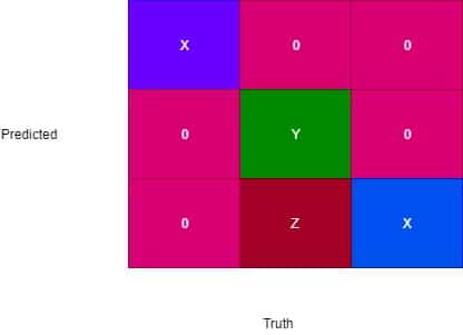
# Plot Confusion Matrix
matp = confusion_matrix(predicted, ztest)
names = nump.unique(predicted)
seb.heatmap(matp, square=True, annot=True, fmt='d', cbar=False,
wticklabels=names, zticklabels=names)
pltt.wlabel('Truth')
pltt.zlabel('Predicted')
How to Improve Your Model
Laplace correction can be used to manage the records with zero for W variables.
You can combine features of products to create a new one and can be known as feature engineering. Here, the Naive Bayes on the assumptions that features are independent. You can check and try to remove the correlated features.
Also, can try to transform the variables to make the features near normal using BoxCox or YeoJohnson like transformations.
For the algorithm based on knowledge, try to provide a realistic probability. To reduce variance you can ensemble methods like boosting, bagging etc. Now, you have a clear idea about how companies are using Naive Bayes algorithm for prediction making and various other decision-making tasks oriented with data. Learning it with other data science algorithms can be very helpful to drive your journey.
Data science is considered as the Highest Paying IT Certifications due to lack of such talents these days. Companies are looking for experts with the art of dealing correlating data and analyzing it. So, it is the golden time for those who are willing to get a stable IT job.